Meaning of conditional probability

Conditional probability was always baffling me. Empirical, frequentists meaning is clear, but the abstract definition, originating from Kolmogorov – what was its mathematical meaning? How it can be derived? It’s a nontrivial definition and is appearing in the textbooks out the air, without measure theory intuition behind it.

Here I mostly follow Chang&Pollard paper Conditioning as disintegartion. Beware that the paper use non-standard notation, but this post follow more common notation, same as in wikipedia.

Here is example form Chang&Pollard paper:

Suppose we have distribution on $\mathbb{R}^2$ concentrated in two straight lines $L_1$ and $L_2$ with respective density $g_i(x)$ and angles with X axis $\alpha_i$ . Observation (X,Y) taken, giving $X=x_0$ , what is probability that point lies on the line $L_1$ ?

Standard approach would be approximate $x_0$ with $[ x_0, x_0 +\Delta ]$ and take limit with $\Delta \to 0$

$\frac{\int_{x_0}^{x_0+ \Delta}g_1/cos(\alpha_1)}{\int_{x_0}^{x_0+ \Delta}g_1/cos(\alpha_1) + \int_{x_0}^{x_0+ \Delta}g_2/cos(\alpha_2)}$

Not only taking this limit is kind of cumbersome, it’s also not totally obvious that it’s the same conditional probability that defined in the abstract definition – we are replacing ratio with limit here.

Now what is “correct way” to define conditional probabilities, especially for distributions?

Disintegration!

For simplicity we will first talk about single scalar random variable, defined on probability space. We will think of random variable X as function on the sample space. Now condition $X=x_0$ define fiber – inverse image of $x_0$ .

Disintegration theorem say that probability measure on the sample space can be decomposed into two measures – parametric family of measures induced by original probability on each fiber and “orthogonal” measure on $\mathbb{R}$ – on the parameter space of the first measure. Here $\mathbb{R}$ is the space of values of X and serve as parameter space for measures on fibers. Second measure induced by the inverse image of the function (random variable) for each measurable set on $\mathbb{R}$ . This second measure is called Pushforward measure. Pushforward measure is just for measurable set on $\mathbb{R}$ (in our case) taking its X inverse image on sample space and measuring it with μ.

Fiber is in fact sample space for conditional event, and measure on fiber is our conditional distribution.

Full statement of the theorem require some term form measure theory. Following wikipedia

Let P(X) is collection of Borel probability measures on X, P(Y) is collection of Borel probability measures on Y

Let Y and X be two Radon spaces. Let μ ∈ P(Y), let $\pi$ : Y → X be a Borel- measurable function, and let ν ∈ P(X) be the pushforward measure $\mu \circ \pi^{-1}$ .

* Then there exists a ν-almost everywhere uniquely determined family of probability measures $\mu_x$ ⊆ P(Y) such that
* the function $x \mapsto \mu_{x}$ is Borel measurable, in the sense that $x \mapsto \mu_{x} (B)$ is a Borel-measurable function for each Borel-measurable set B ⊆ Y;
* $\mu_x$ “lives on” the fiber $\pi^{-1}(x)$ : for ν-almost all x ∈ X,

$\mu_x(Y \setminus \pi^{-1} (x))=0$

and so $\mu_x(E)=\mu_x(E \cap \pi^{-1}(x))$

* for every Borel-measurable function $f$ : Y → [0, ∞],

$\int_{Y} f(y) \, \mathrm{d} \mu (y) = \int_{X} \int_{\pi^{-1} (x)} f(y) \, \mathrm{d} \mu_{x} (y) \mathrm{d} \nu (x)$

From here for any event E form Y

$\mu (E) = \int_{X} \mu_{x} \left( E \right) \, \mathrm{d} \nu (x)$

This was complete statement of the disintegration theorem.

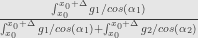
Now returning to Chang&Pollard example. For formal derivation I refer you to the original paper, here we will just “guess” $\mu_x$ , and by uniqueness it give us disintegration. Our conditional distribution for $X=x$ will be just point masses on the intersections of lines $L_1$ and $L_2$ with axis $X=x$
Here $\delta$ is delta function – point mass.

$d\mu_x(y) = \frac{\delta (L_1( x )-y) g_1( x ) / cos(\alpha_1) + \delta (L_2( x )-y) g_2( x ) / cos(\alpha_2)}{Z(x)}dy$

$Z(x) = g_1(x)/cos(\alpha_1) + g_2(x)/cos(\alpha_2)$

and for $\nu$
$d\nu = Z(x)dx$

Our conditional probability that event lies on $L_1$ with condition $X = x_0$ , form conditional density $d\mu_{x_0}/dy$ thus

$\frac{g_1(x_0)/cos(\alpha_1)}{g_1(x_0)/cos(\alpha_1) + g_2(x_0)/cos(\alpha_2)}$

Another example from Chen&Pollard. It relate to sufficient statistics. Term sufficient statistic used if we have probability distribution depending on some parameter, like in maximum likelihood estimation. Sufficient statistic is some function of sample, if it’s possible to estimate parameter of distribution from only values of that function in the best possible way – adding more data form the sample will not give more information about parameter of distribution.
Let $\mathbb{P}_{\theta}$ be uniform distribution on the square $[0, \theta]^2$ . In that case M = max(x, y) is sufficient statistics for $\theta$ . How to show it?
Let take our function $(x,y) \to m$ , $m = max(x,y)$ and make disintegration.
$d\mu_m(x,y) = s_m(x,y)dxdy$ is a uniform distribution on edges where x and y equal m and $d\nu = (2m / \theta^2 )dm$
$s_m(x,y)$ is density of conditional probability $P(\cdot | M = m)$ and it doesn’t depend on $\theta$
For any $f \ \ \mathbb{P}_{\theta}(f| m) = \int f s_m(x,y) \ , \ \mathbb{P}_{\theta, m}(\cdot) = \mathbb{P}_{m}(\cdot)$ – means that M is sufficient.

It seems that in most cases disintegration is not a tool for finding conditional distribution. Instead it can help to guess it and form uniqueness prove that the guess is correct. That correctness could be nontrivial – there are some paradoxes similar to Borel Paradox in Chang&Pollard paper.

7, November, 2013 - Posted by mirror2image | Math | machine learning, Math, Science

Sorry, the comment form is closed at this time.

« Previous | Next »

Mirror Image

Mostly AR and Stuff