Robust estimators III: Into the deep
Cauchy estimator have some nice properties (Gonzales et al “Statistically-Efficient Filtering in Impulsive Environments: Weighted Myriad Filter” 2002):
By tuning 
it can approximate either least squares (big 
Another property is that for several measurements with different scales 
which is convenient for estimation of random walks


I heard convulsion in the sky,
And flight of angel hosts on high,
And monsters moving in the deep
Those verses from The Prophet by A.Pushkin could be seen as metaphor of profound mathematical insight, encompassing bifurcations, higher dimensional algebra and murky depths of statistics.
I now intend to dive deeper into of statistics – toward “data depth”. Data depth is a generalization of median concept to multidimensional data. Remind you that median can be seen either as order parameter – value dividing the higher half of measurements from lower, or geometrically, as the minimum of 
First approach to generalizations of median is to try to apply order statistics to multidimensional vectors.The idea is to make some kind of partial order for n-dimensional points – “depth” of points, and to choose as the analog of median the point of maximum depth.
Basically all data depth concepts define “depth” as some characterization of how deep points are reside inside the point cloud.
Historically first and easiest to understand was convex hull approach – make convex hull of data set, assign points in the hull depth 1, remove it, get convex hull of points remained inside, assign new hull depth 2, remove etc.; repeat until there is no point inside last convex hull.
Later Tukey introduce similar “halfspace depth” concept – for each point X find the minimum number of points which could be cut from the dataset by plane through the point X. That number count as depth(see the nice overview of those and other geometrical definition of depth at Greg Aloupis page)
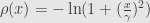
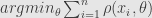
In 2002 Mizera introduced “global depth”, which is less geometric and more statistical. It start with assumption of some loss function (“criterial function” in Mizera definition) 


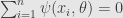
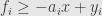
Tangent depth defined as 
Those definitions of “data depth” allow for another type of estimator, based not on likelihood, but on order statistics –maximum depth estimators. The advantage of those estimators is robustness(breakdown point ~25%-33%) and disadvantage – low precision (high bias). So I wouldn’t use them for precise estimation, but for sanity check or initial approximation. In some cases they could be computationally more cheap than M-estimators. As useful side effect they also give some insight into structure of dataset(it seems originally maximum depth estimators was seen as data visualization tool). Depth could be good criterion for outliers rejection.
Disclaimer: while I had very positive experience with Cauchy estimator, data depth is a new thing for me.I have yet to see how useful it could be for computer vision related problems.
Robust estimators II
In this post I was complaining that I don’t know what breakdown point for redescending M-estimators is. Now I found out that upper bound for breakdown point of redescending of M-estimators was given by Mueller in 1995, for linear regression (that is statisticians word for simple estimation of p-dimensional hyperplane):


That only work if the error present only in results of measurements, which is reasonable condition – in most cases we can move random error from x part to y part.
Now which M-estimators attain this upper bound?
The condition is “slow variation”(Mizera and Mueller 1999)
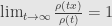
Mentioned in previous post Cauchy estimator is satisfy that condition:
In practice we always work with 

Rule of the thumb: if you don’t know which robust estimator to use, use Cauchy: It’s fast(which is important in real time apps), its easy to understand, it’s differentiable, and it is as robust as possible (that is for redescending M-estimator)

Robust estimators – understand or die… err… be bored trying
This is continuation of my attempt to understand internal mechanics of robust statistics. First I want to say that robust statistics “just works”. It’s not necessary to have deep understanding of it to use it and even to use it creatively. However without that deeper understanding I feel myself kind of blind. I can modify or invent robust estimators empirically, but I can not see clearly the reasons, why use this and not that modification.
Now about robust estimators. They could be divided into two groups: maximum likelihood estimators(M-estimators), which in case of robust statistics usually, but not always are redescending estimators (notable not redescending estimator is
This second “all the rest” group include subset of L-estimators(think of median, which is also M-estimator with
It’s easy to understand what M-estimators do: just find the value of parameter which give maximum probability of given set of measurements.
or
which give us traditional M-estimator form
or
Practically we are usually work not with measurements per se, but with some distribution of cost function 
it’s the same as the previous equation just
Now if we make a set of weights 
We see that it could be considered as “nonlinear least squares”, which could be solved with iteratively reweighted least squares
Now for second group of estimators we have probability of joint distribution
All the global factors – sort order, global scale etc. are incorporated into measurements dependence.
It seems the difference between this formulation of second group of estimators and M-estimator is that conditional independence assumption about measurements is dropped.
Another interesting thing is that if some of measurements are not dependent on others, this formulation can get us bayesian network


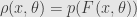
Now lets return to M-estimators. M-estimator is defined by assumption about probability distribution of the measurements.
So M-estimator and probabilistic distribution through which it is defined are essentially the same. Least squares, for example, is produced by normal(gausssian) distribution. Just take sum of logarithms of gaussian and you get least squares estimator.
If we are talking about normal (pun intended), non-robust estimator, their defining feature is finite variance of distribution.
We have central limit theorem which saying that for any distribution mean value of samples will have approximately normal(or Gaussian) distribution.
From this follow property of asymptotic normality – for estimator with finite variance its distribution around true value of parameter
We are discussing robust estimators, which are stable to error and have “thick-tailed” distribution, so we can not assume finite variance of distribution.
Nevertheless to have “true” result we want some form of probabilistic convergence of measurements to true value. As it happens such class of distribution with infinite variance exists. It’s called alpha-stable distributions.
Alpha stable distribution are those distributions for which linear combination of random variables have the same distribution, up to scale factor. From this follow analog of central limit theorem for stable distribution.
The most well known alpha-stable distribution is Cauchy distribution, which correspond to widely used redescending estimator
Cauchy distribution can be generalized in several way, including recent GCD – generalized Cauchy distribution(Carrillo et al), with density function
and estimator
Carrillo also introduce Cauchy distribution-based “norm” (it’s not a real norm obviously) which he called “Lorentzian norm”

He successfully applied Lorentzian norm


Is Robust Statistics have formal mathematical foundation?
As I have already written I have a trouble understanding what robust estimators actually estimate from probabilistic or other formal point of view. I mean estimators which are not maximum likelihood estimators. There is a formal definition which doesn’t explain a lot to me. It looks like estimator estimate some quantity, and we know how good we are at estimating it, but how we know what we are actually estimate? Or does this question even make sense? But that is actually a minor bummer. A problem with understanding outliers is a lot worse for me. A breakdown point is a fundamental concept in robust statistics. And breakdown point is defined as a relative number of outliers in the sample set. The problem is, it seems there is no formal definition of outlier in statistics or probability theory. We can talk about mixture models, and tail distributions but those concepts are not quite consistent with breakdown point. Breakdown point looks like it belong to area of optimization/topology, not statistics. Could it be that outliers could be defined consistently only if we have some additional structural information/constraints beside statistical (distribution)? That inability to reconcile statistics and optimization is a problem which causing cognitive headache for me.
Minimum sum of distance vs L1 and geometric median
All this post is just a more detailed explanation of the end of the previous post.
Assume we want to estimating a state 


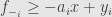
Sharon at al show that minimum
is a robust estimator with stable breakdown point, not depending on the noise level. What Sharon did was to use as cost function the sum of absolute values of all components of errors vector. However there are exists another approach.
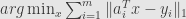
In one-dimensional case minimum 
That is not a least squares – minimized the sum of 
Now why is this a stable and robust estimator? If we look at the Jacobian
we see it’s asymptotically constant, and it’s norm doesn’t depend on the norm of the outliers. While it’s not a formal proof it’s quite intuitive, and can probably be formalized along the lines of Sharon paper.
While first approach with
For interior point method, in both cases original cost function is replaced with
And the value of 

Sometimes it’s formulated by splitting absolute value is into the sum of positive and negative parts


And for
Formulations are very similar, and stability/performance are similar too (there was a paper about it, just had to dig it out)


L1, robust statisrics and compressed sensing
Anyone who did 3D reconstruction and camera pose estimation know, that outliers one of the main, if not the main problem there. There are several ways to deal with outliers, RANSAC and trimming are probably most common. Both of them has major drawback though – they based on the initial error estimation. But for example, in pose estimation, situation where the wrong values have initial error order of magnitude less then correct values is quite common. RANSAC and trimming would make situation worse in that case. What really work there are robust estimators, which is, in many cases just statisticians name for reweighted iterative least square.
Now why and how robust estimators works is really interesting. Basically robust estimator is a maximum likelihood estimator for non-normal distribution, that is distribution with “thick” tail. One of the simplest of robust estimators is L1, which correspond to Laplace distribution. Laplace distribution descend more slow than normal distribution, so it’s obviously more robust. And now the really interesting things start. L1 estimator is the fundamental concept of compressed sensing. And compressed sensing is all about finding “sparse” solution, that is solution which are mostly zeros, but with few components are quite big. And what outliers are? They are exactly “sparse” big components of error vector. If we have linear system with noise in right part, and the noise is dominated by small number of really big outliers then, as Terence Tao pointed out, we can multiply both part of the system on the appropriate matrix and get a sparse system of equations for outliers. That would be a classical compressed sensing problem, for which L1 minimization works perfectly. Recently it was proven, using compressed sensing inspired technique, that L1 estimator for system with outliers really behave similar to L1 minimizer for sparse solutions – it has stable breaking point(Sharon, Wright, Ma, Minimum Sum of Distances Estimator: Robustness and Stability).
That make me think about things I really don’t understand – what is connection between other, redescending estimators and L1 estimator? In practical applications redescending estimators often works better than L1. But redescending estimators practically is not much different form trimming. Does it mean that they are just convenient shortcuts, and in general case L1 is more robust?(One drawback of redescending estimator that it can has multiple local minima) Which assumptions about outliers we should do to to choose most appropriate estimator? I would like to read some theory of redescending estimators, their breaking point and especially their relation to L1, but so far not sure even where to start…
(PPS In this post I talk more about Mueller work on redescending M-estimators which partially answer the question)
PS Another interesting (for me that is, for someone else it could be trivial) problem is dimensionality. For 1-dimensional variable L1 and distance is the same. For vector they are not. So for vector-valued variables estimator “minimum sum of distance” estimator is not the same as L1 estimator. Would be L1 more robust than “minimum sum of distance” for vectors? Compressed sensing logic say that it should, but L1 estimator is anisotropic, it depend on coordinate system. That is for L1 to be effective the outliers should be aligned with coordinate system. Here there is the difference between overall dimensionality of the problem -number of samples and “micro” dimensionality – dimensionality of each sample. I’ll try to sort it out later.
