Deriving Gibbs distribution from stochastic gradients

Stochastic gradients is one of the most important tools in optimization and machine learning (especially for Deep Learning – see for example ConvNet). One of it’s advantage is that it behavior is well understood in general case, by application of methods of statistical mechanics.

In general form stochastic gradient descent could be written as
$w_{n+1} = w_n - \alpha \bigtriangledown E(w_n) + F_n$
where $F_n$ is a random variable with expectation zero.
To apply methods of statistical mechanics we can rewrite it in continuous form, as stochastic gradient flow
$\partial J/\partial t = - \bigtriangledown_J E(J) +F(t)$
and random variable F(t) we assume to be white noise for simplicity.
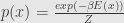
In that moment most of textbooks and papers refer to “methods of statistical mechanics” to show that
stochastic gradient flow has invariant probability distribution, which is called Gibbs distribution
$p(x) = \frac {exp(-\beta E(x))}{Z}$
and from here derive some interesting things like temperature and free energy.
The question is – how Gibbs distribution derived from stochastic gradient flow?

First we have to understand what stochastic gradient flow really means.
It’s not a partial differential equation (PDE), because it include random variable, which is not a function $\mathbb{R} \to \mathbb{R}$ . In fact it’s a stochastic differential equation (SDE) . SDE use some complex mathematical machinery and relate to partial differential equations, probability/statistics, measure theory and ergodic theory. However they used a lot in finance, so there is quite a number of textbooks on SDE for non-mathematicians. For the short, minimalistic and accessible book on stochastic differential equation I can’t recommend highly enough introduction to SDE by L.C. Evans

SDE in question is called Ito diffusion. Solution of that equation is a stochastic process – collection of random variables parametrized by time. Sample path of stochastic process in question as a function of time is nowhere differentiable – it’s difficult to talk about it in term of derivatives, so it is defined through it’s integral form.
First I’ll notice that integral of white noise is actually Brownian motion, or Wiener process.
Assume that we have stochastic differential equation written in informal manner
$\partial X / \partial t = b(X, t) + g(X, t) F(t)$ with X -stochastic process and F(t) – white noise
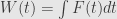
It’s integral form is
$X(T) - X(0) = \int_{0}^{T} b(X, t) dt + \int_{0}^{T} g(X, t) dW(t) \ \ (1)$
where W(t) is a Wiener process
$W(t) = \int F(t) dt$
This equation is usually written in the form
$dX = b(X,t)dt + g(X,t)dW \ \ (2)$
This is only a notation for integral equation, d here is not a differential.
Returning to (1)
$\int_{0}^{T} b(X, t) dt$ is an integral along sample path, it’s meaning is obvious, or it can be defined as limit of Riemann sums with respect to time.

The most notable thing here is
$\int_{0}^{T} g(X, t) dW(t)$ – integral with respect to Wiener process (3)
It’s a stochastic integral, and it’s defined in the courses of stochastic differential equation as the limit of Riemann sums of random variables, in the manner similar to definition of ordinary integral.
Curiously, stochastic integral is not quite well defined. Depending on the form of the sum it produce different results, like Ito integral:

$\int_0^t g \,d W =\lim_{n\rightarrow\infty} \sum_{[t_{i-1},t_i]\in\pi_n}g_{t_{i-1}}(W_{t_i}-W_{t_{i-1}})$
Different Riemann sums produce different integral – Stratonovich integral:
$\int_0^t g \,d W =\lim_{n\rightarrow\infty} \sum_{[t_{i-1},t_i]\in\pi_n}(g_{t_i} + g_{t_{i-1}})/2(W_{t_i}-W_{t_{i-1}})$

Ito integral used more often in statistics because it use $g_{t_{i-1}}$ – it don’t “look forward”, and Stratonovich more used in theoretical physics.

Returning to Ito integral – Ito integral is stochastic process itself, and it has expectation zero for each t.
From definition of Ito integral follow one of the most important tools of stochastic calculus – Ito Lemma (or Ito formula)
Ito lemma states that for solution of SDE (2)
$dX = b(X, t)dt + g(x, t)dW$ X, b, W – vectors, g – matrix
were W is Wiener process (actually some more general process) and b and g are good enough

$du(\mathbf{X}, t) = \frac{\partial u}{\partial t} dt + (\nabla_\mathbf{X}^{\mathsf T} u) d\mathbf{X} + \tfrac{1}{2} \sum_{i,j} (gg^\mathsf{T})_{i,j}\tfrac{ \partial^2 u}{\partial x_i \partial x_j} dt$

where $\nabla_\mathbf{X} u$ is the gradient.
From Ito lemma follow Ito product rule for scalar processes: applying Ito formula to process $V = { X \choose Y}$ combined from two processes X and Y to function u(V) = XY
$d(XY) = XdY + YdX + g_x \cdot g_y dt$
Using Ito formula and Ito product rule it is possible to get Feynman–Kac formula (derivation could be found in the wikipedia, it use only Ito formula, Ito product rule and the fact that expectation of Ito integral (3) is zero):
for partial differential equation (PDE)
$\frac{\partial u}{\partial t} + (\nabla_\mathbf{X}u)^{\mathsf T} b + \tfrac{1}{2} \sum_{i,j} (gg^\mathsf{T})_{i,j}\tfrac{ \partial^2 u}{\partial x_i \partial x_j} - vu = f$
with terminal condition
$u(x, T) = \psi(x) \ \ (4)$
solution can be written as conditional expectation:
$u(x,t) = E\left[ \int_t^T e^{- \int_t^r v(X_\tau,\tau)\, d\tau}f(X_r,r)dr + e^{-\int_t^T v(X_\tau,\tau)\, d\tau}\psi(X_T) \Bigg| X_t=x \right]$
Feynman–Kac formula establish connection between PDE and stochastic process.
From Feynman–Kac formula taking $v\equiv 0$ and $f \equiv 0$ we get Kolmogorov backward equation :
for
$Lu = (\nabla_\mathbf{X}u)^{\mathsf T} b + \tfrac{1}{2} \sum_{i,j} (gg^\mathsf{T})_{i,j}\tfrac{ \partial^2 u}{\partial x_i \partial x_j}$
equation
$\frac{\partial u}{\partial t} + Lu = 0 \ \ (5)$
with terminal condition (4) have solution as conditional expectation
$u(x, t) = E(\psi(X_T) | X_t = x) \ \ (6)$
From Kolmogorov backward equation we can obtain Kolmogorov forward equation, which describe evolution of probability density for random process X (2)
In SDE courses it’s established that (2) is a Markov process and has transitional probability P and transitional density p:
p(x, s, y, t) = probability density at being at y in time t, on condition that it started at x in time s
taking u – solution of (5) with terminal condition (6)
$u(x, s) = E(\psi(X_T) | X_s = x) = \int p(x, s, z, T) \psi(z) dz$
From Markov property
$p(x, s, z, T) = \int p(x, s, y, t)p(y, t, z, T) dz$
from here
$u(x, s) = \int \int p(x, s, y, t) p(y, t, z, T) \psi(z) dz dy$
$u(x, s) = \int p(x, s, y, t) u(y, t) dy$
form here
$0 = \frac{\partial u}{\partial t} = \int \frac {\partial p(x, s, y, t)}{\partial t}u(y, t) + p(x, s, y, t) \frac {\partial u(y, t)}{\partial t} dy$
from (5)
$\int \frac{\partial p(x, s, y, t)}{\partial t}u(y, t) - (Lu) p(x, s, y, t) dy = 0 \ \ (7)$
Now we introduce dual operator $L^*$
$\int p (Lu) dy = \int (L^{*}p) u dy$
By integration by part we can get
$L^*u = -\nabla_\mathbf{X}^{\mathsf T}(ub) + \tfrac{1}{2} \sum_{i,j} \tfrac{ \partial^2 }{\partial x_i \partial x_j}(gg^\mathsf{T}u)_{i,j}$
and from (7)
$\int (\frac{\partial p(x, s, y, t)}{\partial t} - L^{*}p) u(y, t) dy = 0$
for t=T
$\int (\frac{\partial p(x, s, y, T)}{\partial t} - L^{*}p(x, s, y, T)) \psi(y) dy = 0$
This is true for any $\psi$ , wich is independent from p
And we get Kolmogorov forward equation for p. Integrating by x we get the same equation for probability density at any moment T
$\frac{\partial p}{\partial t} - L^{*}p = 0$
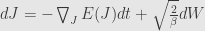
Now we return to Gibbs invariant distribution for gradient flow
$\tfrac{\partial J}{\partial t} = - \bigtriangledown_J E(J) + \sqrt{\tfrac{2}{\beta}}F(t)$
Stochastic gradient flow in SDE notation
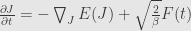
$dJ = - \bigtriangledown_J E(J)dt + \sqrt{\tfrac{2}{\beta}} dW$ – integral of white noise is Wiener process
We want to find invariant probability density $p_G$ . Invariant – means it doesn’t change with time, $\tfrac{\partial p_G}{\partial t} = 0$
so from Kolmogorov forward equation
$L^*p_G = 0$
or
$\nabla^{\mathsf T}(p_G\nabla E)+ \tfrac{1}{\beta} \nabla^{\mathsf T} \nabla p_G = 0$
removing gradient
$p_G\nabla E + \tfrac{1}{\beta} \nabla p_G = C$
C = 0 because we want $p_G$ integrable
$\nabla(E + \tfrac{1}{\beta} log(p_G)) = 0$
and at last we get Gibbs distribution
$p_G = \frac{exp(-\beta E)}{Z}$
Recalling again the chain of reasoning:
Wiener process →