Deriving Gibbs distribution from stochastic gradients
Stochastic gradients is one of the most important tools in optimization and machine learning (especially for Deep Learning – see for example ConvNet). One of it’s advantage is that it behavior is well understood in general case, by application of methods of statistical mechanics.
In general form stochastic gradient descent could be written as
where 
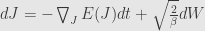
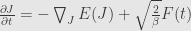
To apply methods of statistical mechanics we can rewrite it in continuous form, as stochastic gradient flow
and random variable F(t) we assume to be white noise for simplicity.
In that moment most of textbooks and papers refer to “methods of statistical mechanics” to show that
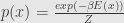
stochastic gradient flow has invariant probability distribution, which is called Gibbs distribution
and from here derive some interesting things like temperature and free energy.
The question is – how Gibbs distribution derived from stochastic gradient flow?


First we have to understand what stochastic gradient flow really means.
It’s not a partial differential equation (PDE), because it include random variable, which is not a function 
SDE in question is called Ito diffusion. Solution of that equation is a stochastic process – collection of random variables parametrized by time. Sample path of stochastic process in question as a function of time is nowhere differentiable – it’s difficult to talk about it in term of derivatives, so it is defined through it’s integral form.
First I’ll notice that integral of white noise is actually Brownian motion, or Wiener process.
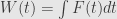
Assume that we have stochastic differential equation written in informal manner

It’s integral form is
where W(t) is a Wiener process
This equation is usually written in the form
This is only a notation for integral equation, d here is not a differential.
Returning to (1)


The most notable thing here is

It’s a stochastic integral, and it’s defined in the courses of stochastic differential equation as the limit of Riemann sums of random variables, in the manner similar to definition of ordinary integral.
Curiously, stochastic integral is not quite well defined. Depending on the form of the sum it produce different results, like Ito integral:
Different Riemann sums produce different integral – Stratonovich integral:
![\int_0^t g \,d W =\lim_{n\rightarrow\infty} \sum_{[t_{i-1},t_i]\in\pi_n}g_{t_{i-1}}(W_{t_i}-W_{t_{i-1}})](https://s0.wp.com/latex.php?latex=%5Cint_0%5Et+g+%5C%2Cd+W+%3D%5Clim_%7Bn%5Crightarrow%5Cinfty%7D+%5Csum_%7B%5Bt_%7Bi-1%7D%2Ct_i%5D%5Cin%5Cpi_n%7Dg_%7Bt_%7Bi-1%7D%7D%28W_%7Bt_i%7D-W_%7Bt_%7Bi-1%7D%7D%29&bg=e6e6e6&fg=333333&s=0&c=20201002)
![\int_0^t g \,d W =\lim_{n\rightarrow\infty} \sum_{[t_{i-1},t_i]\in\pi_n}(g_{t_i} + g_{t_{i-1}})/2(W_{t_i}-W_{t_{i-1}})](https://s0.wp.com/latex.php?latex=%5Cint_0%5Et+g+%5C%2Cd+W+%3D%5Clim_%7Bn%5Crightarrow%5Cinfty%7D+%5Csum_%7B%5Bt_%7Bi-1%7D%2Ct_i%5D%5Cin%5Cpi_n%7D%28g_%7Bt_i%7D+%2B+g_%7Bt_%7Bi-1%7D%7D%29%2F2%28W_%7Bt_i%7D-W_%7Bt_%7Bi-1%7D%7D%29&bg=e6e6e6&fg=333333&s=0&c=20201002)
Ito integral used more often in statistics because it use 
Returning to Ito integral – Ito integral is stochastic process itself, and it has expectation zero for each t.
From definition of Ito integral follow one of the most important tools of stochastic calculus – Ito Lemma (or Ito formula)
Ito lemma states that for solution of SDE (2)

were W is Wiener process (actually some more general process) and b and g are good enough

where 
From Ito lemma follow Ito product rule for scalar processes: applying Ito formula to process 
Using Ito formula and Ito product rule it is possible to get Feynman–Kac formula (derivation could be found in the wikipedia, it use only Ito formula, Ito product rule and the fact that expectation of Ito integral (3) is zero):
for partial differential equation (PDE)
with terminal condition
solution can be written as conditional expectation:
Feynman–Kac formula establish connection between PDE and stochastic process.
From Feynman–Kac formula taking 

for
equation
with terminal condition (4) have solution as conditional expectation
From Kolmogorov backward equation we can obtain Kolmogorov forward equation, which describe evolution of probability density for random process X (2)
In SDE courses it’s established that (2) is a Markov process and has transitional probability P and transitional density p:
p(x, s, y, t) = probability density at being at y in time t, on condition that it started at x in time s
taking u – solution of (5) with terminal condition (6)
From Markov property
from here
form here
from (5)
Now we introduce dual operator
By integration by part we can get
and from (7)
for t=T
This is true for any 
And we get Kolmogorov forward equation for p. Integrating by x we get the same equation for probability density at any moment T
Now we return to Gibbs invariant distribution for gradient flow
Stochastic gradient flow in SDE notation
We want to find invariant probability density 
so from Kolmogorov forward equation
or
removing gradient
C = 0 because we want
and at last we get Gibbs distribution
Recalling again the chain of reasoning:
Wiener process →


![u(x,t) = E\left[ \int_t^T e^{- \int_t^r v(X_\tau,\tau)\, d\tau}f(X_r,r)dr + e^{-\int_t^T v(X_\tau,\tau)\, d\tau}\psi(X_T) \Bigg| X_t=x \right]](https://s0.wp.com/latex.php?latex=u%28x%2Ct%29+%3D+E%5Cleft%5B+%5Cint_t%5ET+e%5E%7B-+%5Cint_t%5Er+v%28X_%5Ctau%2C%5Ctau%29%5C%2C+d%5Ctau%7Df%28X_r%2Cr%29dr+%2B+e%5E%7B-%5Cint_t%5ET+v%28X_%5Ctau%2C%5Ctau%29%5C%2C+d%5Ctau%7D%5Cpsi%28X_T%29+%5CBigg%7C+X_t%3Dx+%5Cright%5D+&bg=e6e6e6&fg=333333&s=0&c=20201002)


SDE + Ito Lemma + Ito product rule + zero expecation of Ito integral →
Kolmogorov backward equation + Markov property of SDE →
Kolmogorov forward equation for probability density →
Meaning of conditional probability
Conditional probability was always baffling me. Empirical, frequentists meaning is clear, but the abstract definition, originating from Kolmogorov – what was its mathematical meaning? How it can be derived? It’s a nontrivial definition and is appearing in the textbooks out the air, without measure theory intuition behind it.
Here I mostly follow Chang&Pollard paper Conditioning as disintegartion. Beware that the paper use non-standard notation, but this post follow more common notation, same as in wikipedia.
Here is example form Chang&Pollard paper:
Suppose we have distribution on 


Standard approach would be approximate 
![[ x_0, x_0 +\Delta ]](https://s0.wp.com/latex.php?latex=%5B+x_0%2C+x_0+%2B%5CDelta+%5D+&bg=e6e6e6&fg=333333&s=0&c=20201002)

Not only taking this limit is kind of cumbersome, it’s also not totally obvious that it’s the same conditional probability that defined in the abstract definition – we are replacing ratio with limit here.
Now what is “correct way” to define conditional probabilities, especially for distributions?
For simplicity we will first talk about single scalar random variable, defined on probability space. We will think of random variable X as function on the sample space. Now condition
Disintegration theorem say that probability measure on the sample space can be decomposed into two measures – parametric family of measures induced by original probability on each fiber and “orthogonal” measure on 
Fiber is in fact sample space for conditional event, and measure on fiber is our conditional distribution.
Full statement of the theorem require some term form measure theory. Following wikipedia
Let P(X) is collection of Borel probability measures on X, P(Y) is collection of Borel probability measures on Y
Let Y and X be two Radon spaces. Let μ ∈ P(Y), let 

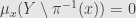
* Then there exists a ν-almost everywhere uniquely determined family of probability measures 
* the function 

* 
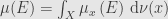
and so
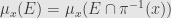
* for every Borel-measurable function 

From here for any event E form Y
This was complete statement of the disintegration theorem.
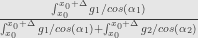
Now returning to Chang&Pollard example. For formal derivation I refer you to the original paper, here we will just “guess” 
Here 


and for


Our conditional probability that event lies on 


Another example from Chen&Pollard. It relate to sufficient statistics. Term sufficient statistic used if we have probability distribution depending on some parameter, like in maximum likelihood estimation. Sufficient statistic is some function of sample, if it’s possible to estimate parameter of distribution from only values of that function in the best possible way – adding more data form the sample will not give more information about parameter of distribution.
Let 
![[0, \theta]^2](https://s0.wp.com/latex.php?latex=%5B0%2C+%5Ctheta%5D%5E2&bg=e6e6e6&fg=333333&s=0&c=20201002)

Let take our function 


For any 

It seems that in most cases disintegration is not a tool for finding conditional distribution. Instead it can help to guess it and form uniqueness prove that the guess is correct. That correctness could be nontrivial – there are some paradoxes similar to Borel Paradox in Chang&Pollard paper.
