Robust estimators II

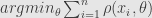
In this post I was complaining that I don’t know what breakdown point for redescending M-estimators is. Now I found out that upper bound for breakdown point of redescending of M-estimators was given by Mueller in 1995, for linear regression (that is statisticians word for simple estimation of p-dimensional hyperplane):

– number of measurements and is little tricky: it is a maximum number of measurement vectors X lying in the same p-dimensional hyperplane. If number of measurements N >> p that mean breakdown point is near 50% – You can have half measurement results completely out of the blue and estimator will still work.
That only work if the error present only in results of measurements, which is reasonable condition – in most cases we can move random error from x part to y part.
Now which M-estimators attain this upper bound?
The condition is “slow variation”(Mizera and Mueller 1999)

Mentioned in previous post Cauchy estimator is satisfy that condition:
and its derivative
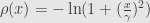
In practice we always work with , not so Cauchy estimator is easy to calculate.
Rule of the thumb: if you don’t know which robust estimator to use, use Cauchy: It’s fast(which is important in real time apps), its easy to understand, it’s differentiable, and it is as robust as possible (that is for redescending M-estimator)

Robust estimators – understand or die… err… be bored trying

This is continuation of my attempt to understand internal mechanics of robust statistics. First I want to say that robust statistics “just works”. It’s not necessary to have deep understanding of it to use it and even to use it creatively. However without that deeper understanding I feel myself kind of blind. I can modify or invent robust estimators empirically, but I can not see clearly the reasons, why use this and not that modification.
Now about robust estimators. They could be divided into two groups: maximum likelihood estimators(M-estimators), which in case of robust statistics usually, but not always are redescending estimators (notable not redescending estimator is norm), and all the rest of estimators.
This second “all the rest” group include subset of L-estimators(think of median, which is also M-estimator with norm.Yea, it’s kind of messy), S-estimators (use global scale estimation for all the measurements) R-estimators, which like L-estimator use order statistics but use it for weights. There may be some others too, but I don’t know much about this second group.
It’s easy to understand what M-estimators do: just find the value of parameter which give maximum probability of given set of measurements.

or

which give us traditional M-estimator form

or
,
Practically we are usually work not with measurements per se, but with some distribution of cost function of the measurements , so it become

it’s the same as the previous equation just defined in such a way as to separate statistical part from cost function part.
Now if we make a set of weights it become

We see that it could be considered as “nonlinear least squares”, which could be solved with iteratively reweighted least squares
Now for second group of estimators we have probability of joint distribution

All the global factors – sort order, global scale etc. are incorporated into measurements dependence.
It seems the difference between this formulation of second group of estimators and M-estimator is that conditional independence assumption about measurements is dropped.
Another interesting thing is that if some of measurements are not dependent on others, this formulation can get us bayesian network

Now lets return to M-estimators. M-estimator is defined by assumption about probability distribution of the measurements.
So M-estimator and probabilistic distribution through which it is defined are essentially the same. Least squares, for example, is produced by normal(gausssian) distribution. Just take sum of logarithms of gaussian and you get least squares estimator.
If we are talking about normal (pun intended), non-robust estimator, their defining feature is finite variance of distribution.
We have central limit theorem which saying that for any distribution mean value of samples will have approximately normal(or Gaussian) distribution.
From this follow property of asymptotic normality – for estimator with finite variance its distribution around true value of parameter approximate normal distribution.
We are discussing robust estimators, which are stable to error and have “thick-tailed” distribution, so we can not assume finite variance of distribution.
Nevertheless to have “true” result we want some form of probabilistic convergence of measurements to true value. As it happens such class of distribution with infinite variance exists. It’s called alpha-stable distributions.
Alpha stable distribution are those distributions for which linear combination of random variables have the same distribution, up to scale factor. From this follow analog of central limit theorem for stable distribution.
The most well known alpha-stable distribution is Cauchy distribution, which correspond to widely used redescending estimator

Cauchy distribution can be generalized in several way, including recent GCD – generalized Cauchy distribution(Carrillo et al), with density function

and estimator

Carrillo also introduce Cauchy distribution-based “norm” (it’s not a real norm obviously) which he called “Lorentzian norm”

is correspond classical Cauchy distribution
He successfully applied Lorentzian norm based basis pursuit to compressed sensing problem, which support idea that compressed sensing and robust statistics are dual each other.

Is Robust Statistics have formal mathematical foundation?

As I have already written I have a trouble understanding what robust estimators actually estimate from probabilistic or other formal point of view. I mean estimators which are not maximum likelihood estimators. There is a formal definition which doesn’t explain a lot to me. It looks like estimator estimate some quantity, and we know how good we are at estimating it, but how we know what we are actually estimate? Or does this question even make sense? But that is actually a minor bummer. A problem with understanding outliers is a lot worse for me. A breakdown point is a fundamental concept in robust statistics. And breakdown point is defined as a relative number of outliers in the sample set. The problem is, it seems there is no formal definition of outlier in statistics or probability theory. We can talk about mixture models, and tail distributions but those concepts are not quite consistent with breakdown point. Breakdown point looks like it belong to area of optimization/topology, not statistics. Could it be that outliers could be defined consistently only if we have some additional structural information/constraints beside statistical (distribution)? That inability to reconcile statistics and optimization is a problem which causing cognitive headache for me.

Minimum sum of distance vs L1 and geometric median

All this post is just a more detailed explanation of the end of the previous post.
Assume we want to estimating a state from noisy linear measurements , , – noise with outliers, like in the paper by Sharon, Wright and Ma Minimum Sum of Distances Estimator: Robustness and Stability
Sharon at al show that minimum norm estimator, that is

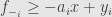
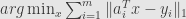
is a robust estimator with stable breakdown point, not depending on the noise level. What Sharon did was to use as cost function the sum of absolute values of all components of errors vector. However there are exists another approach.
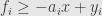
In one-dimensional case minimum norm is a median.But there exist generalization of median to – geometric median. In our case it will be

That is not a least squares – minimized the sum of norm, not the sum of squares of norm.
Now why is this a stable and robust estimator? If we look at the Jacobian

we see it’s asymptotically constant, and it’s norm doesn’t depend on the norm of the outliers. While it’s not a formal proof it’s quite intuitive, and can probably be formalized along the lines of Sharon paper.
While first approach with norm can be solved with linear programming, for example simplex method and interior point method, the second approach with norm can be solved with second order cone programming and …surprise, interior point method again.
For interior point method, in both cases original cost function is replaced with

And the value of is defined by constraints. For
,
Sometimes it’s formulated by splitting absolute value is into the sum of positive and negative parts
, , ,
And for it’s a simple

Formulations are very similar, and stability/performance are similar too (there was a paper about it, just had to dig it out)

L1, robust statisrics and compressed sensing

Anyone who did 3D reconstruction and camera pose estimation know, that outliers one of the main, if not the main problem there. There are several ways to deal with outliers, RANSAC and trimming are probably most common. Both of them has major drawback though – they based on the initial error estimation. But for example, in pose estimation, situation where the wrong values have initial error order of magnitude less then correct values is quite common. RANSAC and trimming would make situation worse in that case. What really work there are robust estimators, which is, in many cases just statisticians name for reweighted iterative least square.
Now why and how robust estimators works is really interesting. Basically robust estimator is a maximum likelihood estimator for non-normal distribution, that is distribution with “thick” tail. One of the simplest of robust estimators is L1, which correspond to Laplace distribution. Laplace distribution descend more slow than normal distribution, so it’s obviously more robust. And now the really interesting things start. L1 estimator is the fundamental concept of compressed sensing. And compressed sensing is all about finding “sparse” solution, that is solution which are mostly zeros, but with few components are quite big. And what outliers are? They are exactly “sparse” big components of error vector. If we have linear system with noise in right part, and the noise is dominated by small number of really big outliers then, as Terence Tao pointed out, we can multiply both part of the system on the appropriate matrix and get a sparse system of equations for outliers. That would be a classical compressed sensing problem, for which L1 minimization works perfectly. Recently it was proven, using compressed sensing inspired technique, that L1 estimator for system with outliers really behave similar to L1 minimizer for sparse solutions – it has stable breaking point(Sharon, Wright, Ma, Minimum Sum of Distances Estimator: Robustness and Stability).
That make me think about things I really don’t understand – what is connection between other, redescending estimators and L1 estimator? In practical applications redescending estimators often works better than L1. But redescending estimators practically is not much different form trimming. Does it mean that they are just convenient shortcuts, and in general case L1 is more robust?(One drawback of redescending estimator that it can has multiple local minima) Which assumptions about outliers we should do to to choose most appropriate estimator? I would like to read some theory of redescending estimators, their breaking point and especially their relation to L1, but so far not sure even where to start…
(PPS In this post I talk more about Mueller work on redescending M-estimators which partially answer the question)

PS Another interesting (for me that is, for someone else it could be trivial) problem is dimensionality. For 1-dimensional variable L1 and distance is the same. For vector they are not. So for vector-valued variables estimator “minimum sum of distance” estimator is not the same as L1 estimator. Would be L1 more robust than “minimum sum of distance” for vectors? Compressed sensing logic say that it should, but L1 estimator is anisotropic, it depend on coordinate system. That is for L1 to be effective the outliers should be aligned with coordinate system. Here there is the difference between overall dimensionality of the problem -number of samples and “micro” dimensionality – dimensionality of each sample. I’ll try to sort it out later.

Visualizing Bundle Adjustment

One of the problem with bundle adjustment is multiple local minimums. If initial approximation is not good enough solution could converge to wrong minima. If this problem arise global optimization should be used. There are several branch and bound bundle adjustment methods for it, which use fractional programming.
Though it’s usually possible to choose correct minima with some geometric consistency check or additional information, I’m trying to understand this situation better. I’ve tried to visualize reprojection error distribution for 2-frame bundle adjustment.
Those pictures represent dependence of reprojection error on the values of second camera position and rotation relatively to first camera.
First, it’s interesting to see how minimal error depend on translational parameter, with fixed rotational parameters. Here 3d structure factored out and translation parametrized with first frame epipole position. Here we see reprojection error depending on the epipole of the first frame only.

This picture easy to understand. “Turbulent” area in the center – the situation where epipole is close to projections of the points. Black tails – area where solution – epipole which minimize reprojection error are situated. It could be seen that epipole have “preferred” direction – the direction from the coordinate center to epipole is more important than distance from center to epipole. There are to “tails” because epipole pass through infinity. This picture also shows that coordinate descent could be effective for factoring out translation, with descent first by direction and second by distance. This wouldn’t work if epipole is near center. The situation where epipole is near center correspond translation of the second camera by mostly Z-axis , but in that case bundle adjustment is not robust anyway.

Now to more complicated problem – visualizing reprojection error parametrized with rotational parametres. 3D structure is factored out as in the first example , and using insight we got in the first example translation parameter approximately factored out with coordinate descent. Two rotational parameters are correspond to projection of the normal to the camera plane of the second camera on the first camera plane. Third parameter (rotation around that normal) is fixed with initial approximation.

Here we see some edgelike artifacts caused by imperfect factoring out translation.
It really should be more smooth, something like that – in this picture epipole distance from the center fixed in infinity. That make picture more smooth but less correct.

Returning to the first rotational parameter example – green pixels mark local minima of the approximation, blue and light blue circles mark two minima to which bundle adjustment actually converge. They dont’ fit approximation exactly, due to error of factoring out epiploes.
What can we see that picture? The local minimums are situated inside connected areas, which generally can be represented as ellipses only poorly (one area is more like spiral). That explain why quadratic methods(Gauss–Newton, Levenberg–Marquardt) are not always work efficiently for bundle adjustment.
The interesting thing is that all area approximately connect in some kind of X-shaped center, where reprojection error locally maximal. I have seen this behavior on other examples too. Right now I don’t understand completely why it happens and what is the nature of this “center”. If this is universal property and this “center” can be efficiently located that effect could be useful.
With multiple frame bundle adjustment situation could be different, but it’s a lot more difficult both to visualize and calculate.
Here are original camera frames, on which bundle adjustment is executed.

More bundle adjustment

Here is some more narrow baseline local bundle adjustment, from only two camera frames.

Outlier is drawn in red. Some points are not detected as outliers, but still are not localized properly.
Multiscale FAST used for detection. No descriptors were used for point correspondence, instead incremental tracking with search in sliding window by average gradient responses was used(there are three tracked frames between those two). I think those bad points could possibly be isolated with some geometric consistency rules, presuming landscape is smooth.

Still checking Gauss-Newton

Though Levenberg-Marquardt works I’m still trying to save Gauss-Newton, especially as I’ve read paper saying that Gauss-Newton with dogleg trust-region works well for bundle adjustment. I’ll probably try direct substitution with Cholesky rank-1 update and constrained optimization.

Solution – free gauge

Looks like the problem was not the large Gauss-Newton residue. The problem was gauge fixing.
Most of bundle adjustment algorithms are not gauge invariant inherently (for details check Triggs “Bundle adjustment – a modern synthesis”, chapter 9 “Gauge Freedom”). Practically that means that method have one or more free parameters which could be chosen arbitrary (for example scale), but which influence solution in non-invariant way (or don’t influence solution if algorithm is gauge invariant). Gauge fixing is the choice of the values for that free parameters. There exist at least one gauge invariant bundle adjustment method (generalization of Levenberg-Marquardt with complete matrix correction instead of diagonal only correction) , but it is order of magnitude more computational expensive.
I’ve used fixing coordinate of one of the 3d points for gauge fixing. Because method is not gauge invariant solution depend on the choice of that fixed point. The problem occurs when the chosen point is “bad” – error in feature point detector for this point is so big that it contradict to the rest of the picture. Mismatching in the point correspondence can cause the same problem.
In my case, fixing coordinate of chosen point caused “accumulation” of residual error in that point. This is easy to explain – other points can decrease reprojection error both by moving/rotating camera and by shifting their coordinates, but fixed point can do it only by moving/rotating camera. It looks like if the point was “bad” from the start it can become even worse next iteration as the error accumulate – positive feedback look causing method become unstable. That’s of cause only my observations, I didn’t do any formal analysis.
The obvious solution is to redistribute residual error among all the points – that mean drop gauge fixing and use free gauge. Free gauge is causing arbitrary scaling of the result, but the result can be rescaled later. However there is the cost. Free gauge means matrix is singular – not invertible and Gauss-Newton method can not work. So I have to switch to less efficient and more computationally expensive Levenberg-Marquardt. For now it seems working.
PS Free gauge matrix is not singular, just not well-defined and has degenerate minimum. So constrained optimization still may works.
PPS Gauge Invariance is also important concept in physics and geometry.
PPPS While messing with Quasi-Newton – it seems there is an error in chapter 10.2 of “Numerical Optimization” by Nocedal&Wright. In the secant equation instead of should be

Problems

During the tests I’ve found out that bundle adjustment is failing on some “bad frames”. There two ways to deal with it – reject bad frames or try to understand what happen – who set up us a bomb? :-).Any problem is also an opportunity to understand subject better. For now I suspect Gauss-Newton is failing due to too big residue. Just adding Hessian to does not help – I’m getting negative eigenvalue. So now I’m trying quasi-Newton from the excellent book by Nocedal&Wright. If it will not help I’ll try hybrid Fletcher method.

PS It looks like the problem was not the large residue