December finds in #arxiv

Repost from my googleplus stream

Computer Vision
Non-Local means is a local image denoising algorithm
Paper shows that non-local mean weights are not identify patches globally point in the images, but are susceptible to aperture problem:
http://en.wikipedia.org/wiki/Optical_flow#Estimation That’s why short radius NLM could be better then large radius NLM. Small radius cutoff play the role of regularizer, similar to the Total Variation in Horn-Shunk Optical flow.
http://en.wikipedia.org/wiki/Horn%E2%80%93Schunck_method (my comment – TV-L1 is generally better than TV-L2 in Horn-Schunk)
http://arxiv.org/abs/1311.3768

Deep Learning
Do Deep Nets Really Need to be Deep?
Authors state that shallow neural nets can in fact achieve similar performance to deep convolutional nets. The problem though is, that they had to be initialized or preconditioned – they can not be trained using existing algorithms.
And for that initialization they need deep nets. Authors hypothesize that there should be algorithms that allow training of those shallow nets to reach the same performance as deep nets.
http://arxiv.org/abs/1312.6184

Intriguing properties of neural networks
The linear combination of deep-level nodes produce the same results as the the original nodes. That  suggest that nodes the spaces itself rather it’s representation keep information for deep levels.
The input-output mapping also discontinuous – small perturbations cause misclassification. Those perturbation are not dependent on the training, only on input of classification. (My comment – sparse coding is generally not smooth on input, another argument that sparse coding is part of internal mechanics of deep learning)
http://arxiv.org/abs/1312.6199

From Maxout to Channel-Out: Encoding Information on Sparse Pathways
This paper start with observation that max-out is a form of sparse coding: only one of the input pathway is chosen for father processing. From this inferred development of that principle:
remove “middle” layer which “choose” maximum input, and transfer maximal input at once into next level – make choice function index-aware. Some other choice function beside the max is considered, but max still seems the best
Piecewise-constant choice function make interesting reference to previous paper (discontinuity of input-output mapping)
http://arxiv.org/abs/1312.1909

Unsupervised Feature Learning by Deep Sparse Coding
This, for a difference is not about convolutional network.
Instead SIFT(or similar) descriptors are used to produce bag-of-words, sparse coding is used with max-out, and manifold learning applied to it. (http://en.wikipedia.org/wiki/Nonlinear_dimensionality_reduction)
http://arxiv.org/abs/1312.5783

Generative NeuroEvolution for Deep Learning
I’m generally wary of evolutionary methods, but this looks kind of interesting –  it’s based on compositional pattern producing network (CPPN)- encoding geometric pattern as composition of simple functions.
This CPPN is used to encode connectivity pattern of ANN (Convolutional newtwork most used). Thus complete process is the combination of ANN training and evolutionary CPPN training
http://arxiv.org/abs/1312.5355

Some Improvements on Deep Convolutional Neural Network Based Image Classification, Unsupervised feature learning by augmenting single images
Botht papers seems about the same subject – squeeze more out of labeled images by applying a lot of transformation to them(Some of those transformations are implemented in cuda-convnet BTW)
http://arxiv.org/abs/1312.5402, http://arxiv.org/abs/1312.5242

Exact solutions to the nonlinear dynamics of learning in deep linear neural networks
Analytical exploration of toy 3-layer model *without_ actual non-linear neurons. Model completely linear to input (polynomial to weights). Nevertheless it show some interesting properties, like step in learning curve
http://arxiv.org/abs/1312.6120

Optimization
Distributed Interior-point Method for Loosely Coupled Problems
Mixing together all my favorite methods: Interior point, Newton, ADMM(Split-Bregman) into one algorithm  and make a distribute implementation of it.
Mixing Newton and ADMM, ADMM and Interior point looks risky to me, though with a lot of subiterations it may work(that’s why it’s distributed – require a lot of calculating power)
Also I’m not sure about convergene of the combined algorithm – each step’s convergence is proven, but I’m not sure the same could be applyed to the combination.
Newton and ADMM have kind of contradicting optimal conditions – smoothness vs piecewise linearity. Would like to see more research on this…
http://arxiv.org/abs/1312.5440

Total variation regularization for manifold-valued data
Proximal mapping and soft thresholding for manifolds – analog of ADMM for manifolds.
http://arxiv.org/abs/1312.7710

just interesting stuff
Coping with Physical Attacks on Random Network Structures
Include finding vulnerable spots and results of random attacks
(My comment – shouldn’t it be connected to precolation theory?)
http://arxiv.org/abs/1312.6189

November finds in #arxiv and NIPS 2013

This is “find in arxiv” reposts form my G+ stream for November.

NIPS 2013

Accelerating Stochastic Gradient Descent using Predictive Variance Reduction

Stochastic gradient (SGD) is the major tool for Deep Learning. However if you look at the plot of cost function over iteration for   SGD you will see that after quite fast descent it becoming extremely slow, and error decrease could even become non-monotonous.  Author explain by necessity of trade of between the step size and variance of random factor – more precision require smaller variance but that mean smaller descent step and slower convergence. “Predictive variance” author suggest to mitigate problem is the same old “adding back the noise” trick, used for example in Split Bregman. Worth reading IMHO.

http://papers.nips.cc/paper/4937-accelerating-stochastic-gradient-descent-using-predictive-variance-reduction

Predicting Parameters in Deep Learning
Output of the first layer of ConvNet is quite smooth, and that could be used for dimensionality reduction, using some dictionary, learned or fixed(just some simple kernel). For ConvNet predicting 75% of parameters with fixed dictionary have negligible effect on accuracy.
http://papers.nips.cc/paper/5025-predicting-parameters-in-deep-learning

Learning a Deep Compact Image Representation for Visual Tracking
Application of ADMM (Alternating Direction Method of Multipliers, of which Split Bregman again one of the prominent examples) to denoising autoencoder with sparsity.
http://papers.nips.cc/paper/5192-learning-a-deep-compact-image-representation-for-visual-tracking

Deep Neural Networks for Object Detection
People from Google are playing with Alex Krizhevsky’s ConvNet
http://papers.nips.cc/paper/5207-deep-neural-networks-for-object-detection

–arxiv (last)–

Are all training examples equally valuable?
It’s intuitively obvious that some training sample are making training process worse. The question is – how to find wich sample should be removed from training? Kind of removing outliers. Authors define “training value” for each sample of binary classifier.
http://arxiv.org/pdf/1311.7080

Finding sparse solutions of systems of polynomial equations via group-sparsity optimization
Finding sparse solution of polynomial system with lifting method.
I still not completely understand why quite weak structure constraint is enough for found approximation to be solution with high probability. It would be obviously precise  for binary 0-1 solution, but why for general sparse?
http://arxiv.org/abs/1311.5871

Semi-Supervised Sparse Coding
Big dataset with small amount of labeled samples – what to do? Use unlabeled samples for sparse representation. And train labeled samples in sparse representation.
http://arxiv.org/abs/1311.6834
From the same author, similar theme – Cross-Domain Sparse Coding
Two domain training – use cross domain data representation to map all the samples from both source and target domains to a data representation space with a common distribution across domains.
http://arxiv.org/abs/1311.7080

Robust Low-rank Tensor Recovery: Models and Algorithms
More of tensor decomposition with trace norm
http://arxiv.org/abs/1311.6182

Complexity of Inexact Proximal Newton methods
Application of Proximal Newton (BFGS) to subset of coordinates each step – active set coordinate descent.
http://arxiv.org/pdf/1311.6547

Computational Complexity of Smooth Differential Equations
Polynomial-memory complexity of ordinary differential equations.
http://arxiv.org/abs/1311.5414

–arxiv (2)–

Deep Learning

Visualizing and Understanding Convolutional Neural Networks
This is exploration of Alex Krizhevsky’s  ConvNet
( https://code.google.com/p/cuda-convnet/ )
using “deconvnet” approach – using deconvolution on output of each layer and visualizing it. Results looks interesting – strting from level 3 it’s something like thersholded edge enchantment, or sketch. Also there are evidences supporting “learn once use everywhere” approach – convnet trained on ImageNet is also effective on other datasets
http://arxiv.org/abs/1311.2901

Unsupervised Learning of Invariant Representations in Hierarchical Architectures
Another paper on why and how deep learning works.
Attempt to build theoretical framework for invariant features in deep learning. Interesting result – Gabor wavelets are optimal filters for simultaneous scale and translation invariance. Relations to sparsity and scattering transform
http://arxiv.org/abs/1311.4158

Computer Vision
An Experimental Comparison of Trust Region and Level Sets
Trust regions method for energy-based segmentation.
Trust region is one of the most important tools in optimization, especially non-convex.
http://en.wikipedia.org/wiki/Trust_region
http://arxiv.org/abs/1311.2102

Blind Deconvolution with Re-weighted Sparsity Promotion
Using reweighted L2 norm for sparsity in blind deconvolution
http://arxiv.org/abs/1311.4029

Optimization

Online universal gradient methods
about  Nesterov’s universal gradient method (
http://www.optimization-online.org/DB_FILE/2013/04/3833.pdf )
It use Bregman distance and related to ADMM.
The paper is application of universal gradient method  to online learning and give bound on regret function.
http://arxiv.org/abs/1311.3832

CS
A Component Lasso
Approximate covariance matrix with block-diagonal matrix and apply Lasso to each block separately
http://arxiv.org/abs/1311.4472

_FuSSO: Functional Shrinkage and Selection Operator
Lasso in functional space with some orthogonal basis_
http://arxiv.org/abs/1311.2234

Non-Convex Compressed Sensing Using Partial Support Information
More of Lp norm for sparse recovery. Reweighted this time.
http://arxiv.org/abs/1311.3773

–arxiv  (1)–

Optimization, CS
Scalable Frames and Convex Geometry
Frame theory is a basis(pun intended) of wavelets theory, compressed sening and overcomplete dictionaries in ML
http://en.wikipedia.org/wiki/Frame_of_a_vector_space
Here is a discussion how to make “tight frame”
http://en.wikipedia.org/wiki/Frame_of_a_vector_space#Tight_frames
from an ordinary frame by scaling m of its components
Interesting geometric insight provided – to do it mcomponents of frame should make “blunt cone”
http://en.wikipedia.org/wiki/Convex_cone#Blunt_and_pointed_cones
http://arxiv.org/abs/1310.8107

Learning Sparsely Used Overcomplete Dictionaries via Alternating Minimization
Some bounds for convergence of dictionary learning. Converge id initial error is O(1/s^2), s- sparcity level
http://arxiv.org/abs/1310.7991

Robust estimators
Robustness of ℓ1 minimization against sparse outliers and its implications in Statistics and Signal Recovery
This is another exploration of L1 estimator. It happens (contrary to common sense) that L1 is not especially robust from “breakdown point” point of view if there is no constraint of noise. However it practical usefulness can be explained that it’s very robust to sparse noise
http://arxiv.org/abs/1310.7637

Numerical
Local Fourier Analysis of Multigrid Methods with Polynomial Smoothers and Aggressive coarsening
Overrelaxaction with Chebyshev weights on the fine grid, with convergence analysis.
http://arxiv.org/abs/1310.8385

Meaning of conditional probability

Conditional probability was always baffling me. Empirical, frequentists meaning is clear, but the abstract definition, originating from Kolmogorov – what was its mathematical meaning? How it can be derived? It’s a nontrivial definition and is appearing in the textbooks out the air, without measure theory intuition behind it.

Here I mostly follow Chang&Pollard  paper  Conditioning as disintegartion. Beware that the paper use non-standard notation, but this post follow more common notation, same as in wikipedia.

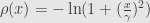
Here is example form Chang&Pollard paper:

Suppose we have distribution on   concentrated in two straight lines  and  with respective density  and angles with X axis . Observation (X,Y) taken, giving , what is probability that point lies on the line  ?

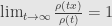
Standard approach would be approximate  with  and take limit with  

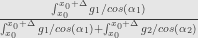
Not only taking this limit is kind of cumbersome, it’s also not totally obvious that it’s the same conditional probability that defined in the abstract definition – we are replacing ratio with limit here.

Now what is “correct way” to define conditional probabilities, especially for distributions?

Disintegration!

For simplicity we will first talk about single scalar random variable, defined on probability space. We will think of random variable X as function on the sample space. Now condition define fiber – inverse image of .

Disintegration theorem say that probability measure on the sample space can be decomposed into two measures – parametric family of measures induced by original probability on each fiber and “orthogonal” measure on  – on the parameter space of the first measure. Here is the space of values of X  and serve as parameter space for measures on fibers. Second measure induced by the inverse image of  the function (random variable) for each measurable set on . This second measure is called Pushforward measure. Pushforward measure is just for measurable set on (in our case) taking its X  inverse image on sample space and measuring it with μ.

Fiber is in fact sample space for conditional event, and measure on fiber is our conditional distribution.

Full statement of the theorem require some term form measure theory. Following wikipedia

Let P(X) is collection of Borel probability measures on X,  P(Y) is collection of  Borel probability measures on Y

Let Y and X be two Radon spaces. Let μ ∈ P(Y), let : Y → X be a Borel- measurable function, and let ν ∈ P(X) be the pushforward measure  .

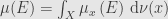
* Then there exists a ν-almost everywhere uniquely determined family of probability measures  ⊆  P(Y) such that
* the function is Borel measurable, in the sense that is a Borel-measurable function for each Borel-measurable set B ⊆ Y;
*    “lives on” the  fiber  : for ν-almost all x  ∈ X,

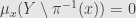
and so

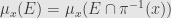
* for every Borel-measurable function : Y → [0, ∞],

From here for any event E form Y

This was complete statement of the disintegration theorem.

Now returning to Chang&Pollard example. For formal derivation I refer you to the original paper, here we will just “guess” , and by uniqueness it give us disintegration. Our conditional distribution for  will be just point masses on the intersections of lines and  with axis  
Here is delta function – point mass.

and for

Our conditional probability that event lies on with condition , form conditional density thus

Another example from Chen&Pollard. It relate to sufficient statistics. Term sufficient statistic used if we have probability distribution depending on some parameter, like in maximum likelihood estimation. Sufficient statistic is some function of sample, if it’s possible to estimate parameter of distribution from only values of that function in the best possible way – adding more data form the sample will not give more information about parameter of distribution.
Let be uniform distribution on the square . In that case M = max(x, y) is sufficient statistics for . How to show it?
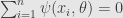
Let take our function , and make disintegration.
is a uniform distribution on edges where x and y equal m and
is density of conditional probability and it doesn’t depend on
For any – means that M is  sufficient.

It seems that in most cases disintegration is not a tool for finding conditional distribution. Instead it can help to guess it and form uniqueness prove that the guess is correct. That correctness could be nontrivial – there are some paradoxes similar to Borel Paradox in Chang&Pollard paper.

Finds in arxiv, october

This is duplication of my ongoing G+ series of post on interesting for me papers in arxiv. Older posts are not here but in my G+ thread.

Finds in #arxiv :
*Optimization, numerical & convex, ML*
The Linearized Bregman Method via Split Feasibility Problems: Analysis and Generalizations
Reformulation of  Split Bregman/ ADMM as split feasibility problem and algorithm/convergence for generalized split feasibility by Bregman projection. This general formulation include both Split Bregman and Kaczmarz (my comment – randomized Kaczmarz  seems could be here too)
http://arxiv.org/abs/1309.2094

Stochastic gradient descent and the randomized Kaczmarz algorithm
Hybrid of  randomized Kaczmarz  and stochastic gradient descent  – into my “to read” pile
http://arxiv.org/abs/1310.5715

Trust–Region Problems with Linear Inequality Constraints: Exact SDP Relaxation, Global Optimality and Robust Optimization
“Extended” trust region for linear inequalities constrains
http://arxiv.org/abs/1309.3000

Conic Geometric Programming
Unifing framwork for conic and geometric programming
http://arxiv.org/abs/1310.0899
http://en.wikipedia.org/wiki/Geometric_programming
http://en.wikipedia.org/wiki/Conic_programming

Gauge optimization, duality, and applications
Another big paper about different, not Lagrange duality, introduced by Freund (1987)
http://arxiv.org/abs/1310.2639

Color Bregman TV
mu parameters in split bregman made adaptive, to exploit coherence of edges in different color channels
http://arxiv.org/abs/1310.3146

Iteration Complexity Analysis of Block Coordinate Descent Methods
Some convergence analysis for BCD and projected gradient BCD
http://arxiv.org/abs/1310.6957

Successive Nonnegative Projection Algorithm for Robust Nonnegative Blind Source Separation
Nonnegative matrix factorization
http://arxiv.org/abs/1310.7529

Scaling SVM and Least Absolute Deviations via Exact Data Reduction
SVN for large-scale problems
http://arxiv.org/abs/1310.7048

Image Restoration using Total Variation with Overlapping Group Sparsity
While title is promising I have doubt about that paper.  The method authors suggest is equivalent to adding averaging filter to TV-L1 under L1 norm. There is no comparison  to just applying TV-L1 and smoothing filter interchangeably.The method author suggest is very costly, and using median filter instead of averaging would cost the same while obviously more robust.
http://arxiv.org/abs/1310.3447

*Deep learning*
Deep and Wide Multiscale Recursive Networks for Robust Image Labeling
_Open source_ matlab/c package coming soon(not yet available)
http://arxiv.org/abs/1310.0354

Improvements to deep convolutional neural networks for LVCSR
convolutional  networks, droput for speech recognition,
http://arxiv.org/abs/1309.1501v1

DeCAF: A Deep Convolutional Activation Feature for Generic Visual Recognition
Already discussed on G+  – open source framework in “learn one use everywhere” stile. Learning done off-line on GPU using ConvNet, and recognition is online in pure python.
http://arxiv.org/abs/1310.1531

Statistical mechanics of complex neural systems and high dimensional data
Big textbook-like overview paper on statistical mechanics of learning. I’ve put it in my “to read” pile.
http://arxiv.org/abs/1301.7115

Randomized co-training: from cortical neurons to machine learning and back again
“Selectron” instead of perception – neurons are “specializing” with weights.
http://arxiv.org/abs/1310.6536

Provable Bounds for Learning Some Deep Representations
http://arxiv.org/abs/1310.6343
Citation:”The current paper presents both an interesting family of denoising autoencoders as

well as new algorithms to provably learn almost all models in this family.”

*Computer vision*
Online Unsupervised Feature Learning for Visual Tracking
Sparse representation, overcomplete dictionary
http://arxiv.org/abs/1310.1690

From Shading to Local Shape
Shape restoration from local shading – could be very useful in low-feature environment.
http://arxiv.org/abs/1310.2916

Fast 3D Salient Region Detection in Medical Images using GPUs
Finding interest point in 3D images
http://arxiv.org/abs/1310.6736

Object Recognition System Design in Computer Vision: a Universal Approach
Grid-based universal framework for object detection/classification
http://arxiv.org/abs/1310.7170

Gaming :)
Lyapunov-based Low-thrust Optimal Orbit Transfer: An approach in Cartesian coordinates
For space sim enthusiast :)
http://arxiv.org/abs/1310.4201

Interior point method – if all you have is a hammer

Interior point method for nonlinear optimization often considered as complex, or highly nontrivial etc. The fact is, that for “simple” nonlinear optimization it’s quite simple, manageable and can even be explained in #3tweets. For those not familiar with it there is a simple introduction to it in wikipedia, which in turn follows an excellent paper by Margaret H. Wright.
Now about “if all you have is a hammer, everything looks like a nail”. Some of applications of interior point method could be quite unexpected.
Everyone who worked with Levenberg-Marquardt minimization algorithm know how much pain is the choice of the small parameter . Levenberg-Marquardt can also be seen as modification of Gauss-newton with a trust region. The of Levenberg-Marquardt do correspond to the trust region radius, but that dependence is highly complex and is difficult to estimate. You want trust region of the radius r, but what should be avlue of ? There is no easy answer to that question; there are some complex methods, or there is a testing with subdivision, which is what the original Levenberg-Marquardt implement.
Interior point can help here.
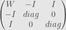
If we choose shape of trust region for Gauss-Newton as hypercube or simplex or like, we can formulate it as set of L1 norm inequality constrains. And that is the domain of interior point method! For hypercube the resulting equations looks especially nice

W – hessian, I – identity, diag – diagonal
That is a banded arrowhead matrix, and for it Cholesky decomposition cost insignificantly more than decomposition of original W. The matrix is not positive definite – Cholesky without square root should be used.
Now there is a temptation to use single constrain instead of set of constrain , but that will not work. should have to be linearized to be tractable, but it’s a second order condition – it’s linear part is zero, so linearization doesn’t constrain anything.
The same method could be used whenever we have to put constrain on the value of Gauss-Newton update, and shape of constrain in not important (or polygonal)
Now last touch – Interior point method has small parameter of it’s own. It’s called usually . In the “normal” method there is a nice rule for it update – take it as (in the notation from wikipedia article – is a value of constraint, is a value of slack variable at the previous iteration) That rule usually explicitly stated in the articles about Interior Point Method(IPM) for Linear Programming, but omitted (as obvious probably) in the papers about IPM for nonlinear optimization
In our case (IPM for trust region) we don’t need update at all – we move boundary of the region with each iteration, so each is an initial value. Have to remember, is not a size of trust region, but strength of it’s enforcement.

Effectivness of compressed sensing in image processing and other stuff

I seldom post in the this blog now, mostly because I’m positing on twitter and G+ a lot lately. I still haven’t figured out which post should go where – blog, G+ or twitter, so it’s kind of chaotic for now.
What of interest is going on: There are two paper on the CVPR11 which claim that compressed sensing(sparse recovery) is not applicable to some of the most important computer vision tasks:
Is face recognition really a Compressive Sensing problem?
Are Sparse Representations Really Relevant for Image Classification?
Both paper claim that space of the natural images(or their important subsets) are not really sparse.
Those claims however dont’t square with claim of high effectiveness of compact signature of Random Ferns.
Could both of those be true? In my opinion – yes. Difference of two approaches is that first two paper assumed explicit sparsity – that is they enforced sparsity on the feature vector. Compressed signature approach used implicit sparsity – feature vector underling the signature is assumed sparse but is not explicitly reconstructed. Why compressed signature is working while explicit approach didn’t? That could be the case if image space is sparse in the different coordinate system – that is here one is dealing with the union of subspaces. Assumption not of the simple sparsity, but of the union of subspaces is called blind compressed sensing.
Now if we look at the space of the natural images it’s easy to see why it is low dimensional. Natural image is the image of some scene, an that scene has limited number of moving object. So dimension of space images of the scene is approximately the sum of degree of freedom of the objects(and camera) of the scene, plus effects of occlusions, illumination and noise. Now if the add strong enough random error to the scene, the image is stop to be the natural image(that is image of any scene). That mean manifold of the images of the scene is isolated – there is no natural images in it’s neighborhood. That hint that up to some error the space of the natural images is at least is the union of isolated low-dimensional manifolds. The union of mainfolds is obviously is more complex structure than the union of subspace, but methods of blind compressed sensing could be applicable to it too. Of cause to think about union of manifolds could be necessary only if the space of images is not union of subspace, which is obviously preferable case

Robust estimators III: Into the deep

Cauchy estimator have some nice properties (Gonzales et al “Statistically-Efficient Filtering in Impulsive Environments: Weighted Myriad Filter” 2002):
By tuning in

it can approximate either least squares (big ), or mode – maximum of histogram – of sample set (small ). For small estimator behave the same way as power law distribution estimator with small .
Another property is that for several measurements with different scales estimator of their sum will be simple

which is convenient for estimation of random walks

I heard convulsion in the sky,
And flight of angel hosts on high,
And monsters moving in the deep

Those verses from The Prophet by A.Pushkin could be seen as metaphor of profound mathematical insight, encompassing bifurcations, higher dimensional algebra and murky depths of statistics.
I now intend to dive deeper into of statistics – toward “data depth”. Data depth is a generalization of median concept to multidimensional data. Remind you that median can be seen either as order parameter – value dividing the higher half of measurements from lower, or geometrically, as the minimum of norm. Second approach lead to geometric median, about which I already talked about.
First approach to generalizations of median is to try to apply order statistics to multidimensional vectors.The idea is to make some kind of partial order for n-dimensional points – “depth” of points, and to choose as the analog of median the point of maximum depth.
Basically all data depth concepts define “depth” as some characterization of how deep points are reside inside the point cloud.
Historically first and easiest to understand was convex hull approach – make convex hull of data set, assign points in the hull depth 1, remove it, get convex hull of points remained inside, assign new hull depth 2, remove etc.; repeat until there is no point inside last convex hull.
Later Tukey introduce similar “halfspace depth” concept – for each point X find the minimum number of points which could be cut from the dataset by plane through the point X. That number count as depth(see the nice overview of those and other geometrical definition of depth at Greg Aloupis page)
In 2002 Mizera introduced “global depth”, which is less geometric and more statistical. It start with assumption of some loss function (“criterial function” in Mizera definition) of measurement set . This function could be(but not necessary) cumulative probability distribution. Now for two parameters and , is more fit with respect if for all . is weakly optimal with respect to if there is nor better fit parameter with respect to . At last global depth of is the minimum possible size of such that is not weakly optimal with respect to – reminder of measurements. In other words global depth is minimum number of measurements which should be removed for stop being weakly optimal. Global depth is not easy to calculate or visualize, so Mizera introduce more simple concept – tangent depth.
Tangent depth defined as . What does it mean? Tangent depth is minimum number of “bad” points – such points that for specific direction loss function for themis growing.
Those definitions of “data depth” allow for another type of estimator, based not on likelihood, but on order statistics –maximum depth estimators. The advantage of those estimators is robustness(breakdown point ~25%-33%) and disadvantage – low precision (high bias). So I wouldn’t use them for precise estimation, but for sanity check or initial approximation. In some cases they could be computationally more cheap than M-estimators. As useful side effect they also give some insight into structure of dataset(it seems originally maximum depth estimators was seen as data visualization tool). Depth could be good criterion for outliers rejection.
Disclaimer: while I had very positive experience with Cauchy estimator, data depth is a new thing for me.I have yet to see how useful it could be for computer vision related problems.

Robust estimators II

In this post I was complaining that I don’t know what breakdown point for redescending M-estimators is. Now I found out that upper bound for breakdown point of redescending of M-estimators was given by Mueller in 1995, for linear regression (that is statisticians word for simple estimation of p-dimensional hyperplane):

– number of measurements and is little tricky: it is a maximum number of measurement vectors X lying in the same p-dimensional hyperplane. If number of measurements N >> p that mean breakdown point is near 50% – You can have half measurement results completely out of the blue and estimator will still work.
That only work if the error present only in results of measurements, which is reasonable condition – in most cases we can move random error from x part to y part.
Now which M-estimators attain this upper bound?
The condition is “slow variation”(Mizera and Mueller 1999)

Mentioned in previous post Cauchy estimator is satisfy that condition:
and its derivative
In practice we always work with , not so Cauchy estimator is easy to calculate.
Rule of the thumb: if you don’t know which robust estimator to use, use Cauchy: It’s fast(which is important in real time apps), its easy to understand, it’s differentiable, and it is as robust as possible (that is for redescending M-estimator)

Robust estimators – understand or die… err… be bored trying

This is continuation of my attempt to understand internal mechanics of robust statistics. First I want to say that robust statistics “just works”. It’s not necessary to have deep understanding of it to use it and even to use it creatively. However without that deeper understanding I feel myself kind of blind. I can modify or invent robust estimators empirically, but I can not see clearly the reasons, why use this and not that modification.
Now about robust estimators. They could be divided into two groups: maximum likelihood estimators(M-estimators), which in case of robust statistics usually, but not always are redescending estimators (notable not redescending estimator is norm), and all the rest of estimators.
This second “all the rest” group include subset of L-estimators(think of median, which is also M-estimator with norm.Yea, it’s kind of messy), S-estimators (use global scale estimation for all the measurements) R-estimators, which like L-estimator use order statistics but use it for weights. There may be some others too, but I don’t know much about this second group.
It’s easy to understand what M-estimators do: just find the value of parameter which give maximum probability of given set of measurements.

or

which give us traditional M-estimator form

or
,
Practically we are usually work not with measurements per se, but with some distribution of cost function of the measurements , so it become

it’s the same as the previous equation just defined in such a way as to separate statistical part from cost function part.
Now if we make a set of weights it become

We see that it could be considered as “nonlinear least squares”, which could be solved with iteratively reweighted least squares
Now for second group of estimators we have probability of joint distribution

All the global factors – sort order, global scale etc. are incorporated into measurements dependence.
It seems the difference between this formulation of second group of estimators and M-estimator is that conditional independence assumption about measurements is dropped.
Another interesting thing is that if some of measurements are not dependent on others, this formulation can get us bayesian network

Now lets return to M-estimators. M-estimator is defined by assumption about probability distribution of the measurements.
So M-estimator and probabilistic distribution through which it is defined are essentially the same. Least squares, for example, is produced by normal(gausssian) distribution. Just take sum of logarithms of gaussian and you get least squares estimator.
If we are talking about normal (pun intended), non-robust estimator, their defining feature is finite variance of distribution.
We have central limit theorem which saying that for any distribution mean value of samples will have approximately normal(or Gaussian) distribution.
From this follow property of asymptotic normality – for estimator with finite variance its distribution around true value of parameter approximate normal distribution.
We are discussing robust estimators, which are stable to error and have “thick-tailed” distribution, so we can not assume finite variance of distribution.
Nevertheless to have “true” result we want some form of probabilistic convergence of measurements to true value. As it happens such class of distribution with infinite variance exists. It’s called alpha-stable distributions.
Alpha stable distribution are those distributions for which linear combination of random variables have the same distribution, up to scale factor. From this follow analog of central limit theorem for stable distribution.
The most well known alpha-stable distribution is Cauchy distribution, which correspond to widely used redescending estimator

Cauchy distribution can be generalized in several way, including recent GCD – generalized Cauchy distribution(Carrillo et al), with density function

and estimator

Carrillo also introduce Cauchy distribution-based “norm” (it’s not a real norm obviously) which he called “Lorentzian norm”

is correspond classical Cauchy distribution
He successfully applied Lorentzian norm based basis pursuit to compressed sensing problem, which support idea that compressed sensing and robust statistics are dual each other.

Is Robust Statistics have formal mathematical foundation?

As I have already written I have a trouble understanding what robust estimators actually estimate from probabilistic or other formal point of view. I mean estimators which are not maximum likelihood estimators. There is a formal definition which doesn’t explain a lot to me. It looks like estimator estimate some quantity, and we know how good we are at estimating it, but how we know what we are actually estimate? Or does this question even make sense? But that is actually a minor bummer. A problem with understanding outliers is a lot worse for me. A breakdown point is a fundamental concept in robust statistics. And breakdown point is defined as a relative number of outliers in the sample set. The problem is, it seems there is no formal definition of outlier in statistics or probability theory. We can talk about mixture models, and tail distributions but those concepts are not quite consistent with breakdown point. Breakdown point looks like it belong to area of optimization/topology, not statistics. Could it be that outliers could be defined consistently only if we have some additional structural information/constraints beside statistical (distribution)? That inability to reconcile statistics and optimization is a problem which causing cognitive headache for me.