nonlinear optimization « Mirror Image

Finds in arxiv, January.

Repost from googleplus stream

Finds in arxiv

Computer vision
Convex Relaxations of SE(2) and SE(3) for Visual Pose Estimation
Finding camera position from the series of 2D (or depth) images is one of the most common (and difficult) task of computer vision.
The biggest problem here is incorporating rotation into cost(energy) function, that should minimize reprojection(fro 2D) error (seehttp://en.wikipedia.org/wiki/Bundle_adjustment). Usually it’s done by minimization on manifold – locally presenting rotation parameter space as linear subspace. The problem with that approach is that initial approximation should be good enough and minimization goes by small steps pojecting/reprojecting on manifold (SO(3) in the case) which can stuck in local minimum. Where to start if the is no initial approximation? Usually it’s just brute-forced with several initialization attempt. Here in the paper approach is different – no initial approximation needed, solution is straightforward and minimum is global. The idea is instead of minimizing rotation on the sphere minimize it inside the ball. In fact it’s a classical convexification approach – increase dimentionality of the problem to make it convex. The pay is a lot higher computational cost of cause
http://arxiv.org/abs/1401.3700

A Sparse Outliers Iterative Removal Algorithm to Model the Background in the Video Sequences
Background removal without nuclear norm. Some “good” frames chosen as dictionary and backround represented in it.
http://arxiv.org/abs/1401.6013

Deep Learning

Learning Mid-Level Features and Modeling Neuron Selectivity for Image Classification
Mid level features is a relatively new concept but a very old practice. It’s a building “efficient” subset of features from the set of features obtained by low-level feature descriptor(like SIFT, SURF, FREAK etc) Before it was done by PCA, later by sparse coding.
What authors built is some kind of hibrid of convolutional network with dictionary learning. Mid level features fed into neuron layer for sparsification and result into classifier. There are some benchmarks but no CIFAR or MINST
http://arxiv.org/abs/1401.5535

Optimization and CS

Alternating projections and coupling slope
Finding intersection of two non-convex sets with alternating projection. I didn’t new that transversality condition used a lot in convex geometry too.
http://arxiv.org/abs/1401.7569
Bayesian Pursuit Algorithms
Bayesian version of hard thresholding. Bayesian approach is in how threshold is chosen and update scaled.
http://arxiv.org/abs/1401.7538

1, February, 2014 Posted by mirror2image | arxiv | arxiv, compressed sensing, computer vision, Deep Learning, nonlinear optimization | Comments Off on Finds in arxiv, January.

November finds in #arxiv and NIPS 2013

This is “find in arxiv” reposts form my G+ stream for November.

NIPS 2013

Accelerating Stochastic Gradient Descent using Predictive Variance Reduction

Stochastic gradient (SGD) is the major tool for Deep Learning. However if you look at the plot of cost function over iteration for SGD you will see that after quite fast descent it becoming extremely slow, and error decrease could even become non-monotonous. Author explain by necessity of trade of between the step size and variance of random factor – more precision require smaller variance but that mean smaller descent step and slower convergence. “Predictive variance” author suggest to mitigate problem is the same old “adding back the noise” trick, used for example in Split Bregman. Worth reading IMHO.

http://papers.nips.cc/paper/4937-accelerating-stochastic-gradient-descent-using-predictive-variance-reduction

Predicting Parameters in Deep Learning
Output of the first layer of ConvNet is quite smooth, and that could be used for dimensionality reduction, using some dictionary, learned or fixed(just some simple kernel). For ConvNet predicting 75% of parameters with fixed dictionary have negligible effect on accuracy.
http://papers.nips.cc/paper/5025-predicting-parameters-in-deep-learning

Learning a Deep Compact Image Representation for Visual Tracking
Application of ADMM (Alternating Direction Method of Multipliers, of which Split Bregman again one of the prominent examples) to denoising autoencoder with sparsity.
http://papers.nips.cc/paper/5192-learning-a-deep-compact-image-representation-for-visual-tracking

Deep Neural Networks for Object Detection
People from Google are playing with Alex Krizhevsky’s ConvNet
http://papers.nips.cc/paper/5207-deep-neural-networks-for-object-detection

–arxiv (last)–

Are all training examples equally valuable?
It’s intuitively obvious that some training sample are making training process worse. The question is – how to find wich sample should be removed from training? Kind of removing outliers. Authors define “training value” for each sample of binary classifier.
http://arxiv.org/pdf/1311.7080

Finding sparse solutions of systems of polynomial equations via group-sparsity optimization
Finding sparse solution of polynomial system with lifting method.
I still not completely understand why quite weak structure constraint is enough for found approximation to be solution with high probability. It would be obviously precise for binary 0-1 solution, but why for general sparse?
http://arxiv.org/abs/1311.5871

Semi-Supervised Sparse Coding
Big dataset with small amount of labeled samples – what to do? Use unlabeled samples for sparse representation. And train labeled samples in sparse representation.
http://arxiv.org/abs/1311.6834
From the same author, similar theme – Cross-Domain Sparse Coding
Two domain training – use cross domain data representation to map all the samples from both source and target domains to a data representation space with a common distribution across domains.
http://arxiv.org/abs/1311.7080

Robust Low-rank Tensor Recovery: Models and Algorithms
More of tensor decomposition with trace norm
http://arxiv.org/abs/1311.6182

Complexity of Inexact Proximal Newton methods
Application of Proximal Newton (BFGS) to subset of coordinates each step – active set coordinate descent.
http://arxiv.org/pdf/1311.6547

Computational Complexity of Smooth Differential Equations
Polynomial-memory complexity of ordinary differential equations.
http://arxiv.org/abs/1311.5414

–arxiv (2)–

Deep Learning

Visualizing and Understanding Convolutional Neural Networks
This is exploration of Alex Krizhevsky’s ConvNet
( https://code.google.com/p/cuda-convnet/ )
using “deconvnet” approach – using deconvolution on output of each layer and visualizing it. Results looks interesting – strting from level 3 it’s something like thersholded edge enchantment, or sketch. Also there are evidences supporting “learn once use everywhere” approach – convnet trained on ImageNet is also effective on other datasets
http://arxiv.org/abs/1311.2901

Unsupervised Learning of Invariant Representations in Hierarchical Architectures
Another paper on why and how deep learning works.
Attempt to build theoretical framework for invariant features in deep learning. Interesting result – Gabor wavelets are optimal filters for simultaneous scale and translation invariance. Relations to sparsity and scattering transform
http://arxiv.org/abs/1311.4158

Computer Vision
An Experimental Comparison of Trust Region and Level Sets
Trust regions method for energy-based segmentation.
Trust region is one of the most important tools in optimization, especially non-convex.
http://en.wikipedia.org/wiki/Trust_region
http://arxiv.org/abs/1311.2102

Blind Deconvolution with Re-weighted Sparsity Promotion
Using reweighted L2 norm for sparsity in blind deconvolution
http://arxiv.org/abs/1311.4029

Optimization

Online universal gradient methods
about Nesterov’s universal gradient method (
http://www.optimization-online.org/DB_FILE/2013/04/3833.pdf )
It use Bregman distance and related to ADMM.
The paper is application of universal gradient method to online learning and give bound on regret function.
http://arxiv.org/abs/1311.3832

CS
A Component Lasso
Approximate covariance matrix with block-diagonal matrix and apply Lasso to each block separately
http://arxiv.org/abs/1311.4472

_FuSSO: Functional Shrinkage and Selection Operator
Lasso in functional space with some orthogonal basis_
http://arxiv.org/abs/1311.2234

Non-Convex Compressed Sensing Using Partial Support Information
More of Lp norm for sparse recovery. Reweighted this time.
http://arxiv.org/abs/1311.3773

–arxiv (1)–

Optimization, CS
Scalable Frames and Convex Geometry
Frame theory is a basis(pun intended) of wavelets theory, compressed sening and overcomplete dictionaries in ML
http://en.wikipedia.org/wiki/Frame_of_a_vector_space
Here is a discussion how to make “tight frame”
http://en.wikipedia.org/wiki/Frame_of_a_vector_space#Tight_frames
from an ordinary frame by scaling m of its components
Interesting geometric insight provided – to do it mcomponents of frame should make “blunt cone”
http://en.wikipedia.org/wiki/Convex_cone#Blunt_and_pointed_cones
http://arxiv.org/abs/1310.8107

Learning Sparsely Used Overcomplete Dictionaries via Alternating Minimization
Some bounds for convergence of dictionary learning. Converge id initial error is O(1/s^2), s- sparcity level
http://arxiv.org/abs/1310.7991

Robust estimators
Robustness of ℓ1 minimization against sparse outliers and its implications in Statistics and Signal Recovery
This is another exploration of L1 estimator. It happens (contrary to common sense) that L1 is not especially robust from “breakdown point” point of view if there is no constraint of noise. However it practical usefulness can be explained that it’s very robust to sparse noise
http://arxiv.org/abs/1310.7637

Numerical
Local Fourier Analysis of Multigrid Methods with Polynomial Smoothers and Aggressive coarsening
Overrelaxaction with Chebyshev weights on the fine grid, with convergence analysis.
http://arxiv.org/abs/1310.8385

1, December, 2013 Posted by mirror2image | arxiv | arxiv, compressed sensing, Deep Learning, machine learning, Math, nonlinear optimization | Comments Off on November finds in #arxiv and NIPS 2013

Interior point method – if all you have is a hammer

Interior point method for nonlinear optimization often considered as complex, or highly nontrivial etc. The fact is, that for “simple” nonlinear optimization it’s quite simple, manageable and can even be explained in #3tweets. For those not familiar with it there is a simple introduction to it in wikipedia, which in turn follows an excellent paper by Margaret H. Wright.
Now about “if all you have is a hammer, everything looks like a nail”. Some of applications of interior point method could be quite unexpected.
Everyone who worked with Levenberg-Marquardt minimization algorithm know how much pain is the choice of the small parameter $\lambda$ . Levenberg-Marquardt can also be seen as modification of Gauss-newton with a trust region. The $\lambda$ of Levenberg-Marquardt do correspond to the trust region radius, but that dependence is highly complex and is difficult to estimate. You want trust region of the radius r, but what should be avlue of $\lambda$ ? There is no easy answer to that question; there are some complex methods, or there is a testing with subdivision, which is what the original Levenberg-Marquardt implement.
Interior point can help here.
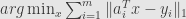
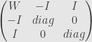
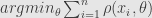
If we choose shape of trust region for Gauss-Newton as hypercube or simplex or like, we can formulate it as set of L1 norm inequality constrains. And that is the domain of interior point method! For hypercube $||\Delta x||_1 \leq \epsilon$ the resulting equations looks especially nice
$\begin{pmatrix} W & -I & I \\ -I & diag & 0 \\ I & 0 & diag \end{pmatrix}$
W – hessian, I – identity, diag – diagonal
That is a banded arrowhead matrix, and for it Cholesky decomposition cost insignificantly more than decomposition of original W. The matrix is not positive definite – Cholesky without square root should be used.
Now there is a temptation to use single constrain $||\Delta x||_2 \leq \epsilon$ instead of set of constrain $||\Delta x||_1 \leq \epsilon$ , but that will not work. $||\Delta x||_2 \leq \epsilon$ should have to be linearized to be tractable, but it’s a second order condition – it’s linear part is zero, so linearization doesn’t constrain anything.
The same method could be used whenever we have to put constrain on the value of Gauss-Newton update, and shape of constrain in not important (or polygonal)
Now last touch – Interior point method has small parameter of it’s own. It’s called usually $\mu$ . In the “normal” method there is a nice rule for it update – take it as $\mu = \lambda C$ (in the notation from wikipedia article – $C$ is a value of constraint, $\lambda$ is a value of slack variable at the previous iteration) That rule usually explicitly stated in the articles about Interior Point Method(IPM) for Linear Programming, but omitted (as obvious probably) in the papers about IPM for nonlinear optimization
In our case (IPM for trust region) we don’t need update $\mu$ at all – we move boundary of the region with each iteration, so each $\mu$ is an initial value. Have to remember, $\mu$ is not a size of trust region, but strength of it’s enforcement.

4, September, 2011 Posted by mirror2image | computer vision, sci | Interior point method, Math, nonlinear optimization | Comments Off on Interior point method – if all you have is a hammer

Robust estimators – understand or die… err… be bored trying

This is continuation of my attempt to understand internal mechanics of robust statistics. First I want to say that robust statistics “just works”. It’s not necessary to have deep understanding of it to use it and even to use it creatively. However without that deeper understanding I feel myself kind of blind. I can modify or invent robust estimators empirically, but I can not see clearly the reasons, why use this and not that modification.
Now about robust estimators. They could be divided into two groups: maximum likelihood estimators(M-estimators), which in case of robust statistics usually, but not always are redescending estimators (notable not redescending estimator is $L_1$ norm), and all the rest of estimators.
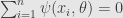
This second “all the rest” group include subset of L-estimators(think of median, which is also M-estimator with $L_1$ norm.Yea, it’s kind of messy), S-estimators (use global scale estimation for all the measurements) R-estimators, which like L-estimator use order statistics but use it for weights. There may be some others too, but I don’t know much about this second group.
It’s easy to understand what M-estimators do: just find the value of parameter which give maximum probability of given set of measurements.
$argmax_{\theta} \prod_{i=1}^{n}p ( x_i\mid\theta)$
or
$argmin_{\theta}\sum_{i=1}^{n} -ln(p(x_i|\theta))$
which give us traditional M-estimator form
$argmin_{\theta}\sum_{i=1}^n \rho(x_i, \theta)$
or
$\sum_{i=1}^n \psi(x_i, \theta) = 0$ , $\psi = \frac{\partial \rho}{\partial \theta}$
Practically we are usually work not with measurements per se, but with some distribution of cost function $F(x,\theta)$ of the measurements $\rho(x, \theta) = p(F(x, \theta))$ , so it become
$\sum_{i=1}^n \psi(x_i, \theta)\frac{\partial F(x_i,\theta)}{\partial \theta} = 0$
it’s the same as the previous equation just $\psi$ defined in such a way as to separate statistical part from cost function part.
Now if we make a set of weights $w_i = \frac{\psi_i}{F_i}$ it become
$\sum_{i=1}^n w_i(x_i, \theta) F(x_i, \theta) \frac{\partial F(x_i,\theta)}{\partial \theta} = 0$
We see that it could be considered as “nonlinear least squares”, which could be solved with iteratively reweighted least squares
Now for second group of estimators we have probability of joint distribution
$argmax_{\theta} \prod_{i=1}^{n}p ( x_i\mid x_{j, j\neq i}, \theta)$
All the global factors – sort order, global scale etc. are incorporated into measurements dependence.
It seems the difference between this formulation of second group of estimators and M-estimator is that conditional independence assumption about measurements is dropped.
Another interesting thing is that if some of measurements are not dependent on others, this formulation can get us bayesian network

Now lets return to M-estimators. M-estimator is defined by assumption about probability distribution of the measurements.
So M-estimator and probabilistic distribution through which it is defined are essentially the same. Least squares, for example, is produced by normal(gausssian) distribution. Just take sum of logarithms of gaussian and you get least squares estimator.
If we are talking about normal (pun intended), non-robust estimator, their defining feature is finite variance of distribution.
We have central limit theorem which saying that for any distribution mean value of samples will have approximately normal(or Gaussian) distribution.
From this follow property of asymptotic normality – for estimator with finite variance its distribution around true value of parameter $\theta$ approximate normal distribution.
We are discussing robust estimators, which are stable to error and have “thick-tailed” distribution, so we can not assume finite variance of distribution.
Nevertheless to have “true” result we want some form of probabilistic convergence of measurements to true value. As it happens such class of distribution with infinite variance exists. It’s called alpha-stable distributions.
Alpha stable distribution are those distributions for which linear combination of random variables have the same distribution, up to scale factor. From this follow analog of central limit theorem for stable distribution.
The most well known alpha-stable distribution is Cauchy distribution, which correspond to widely used redescending estimator
$\psi(x) = \frac {x} {\varepsilon + x^2}$
Cauchy distribution can be generalized in several way, including recent GCD – generalized Cauchy distribution(Carrillo et al), with density function
$p\Gamma(p/2)/2\Gamma(1/p)^2(\sigma^p + x^p)^{-2/p}$
and estimator
$\psi(x)=\frac{p|x|^{p-1}sgn(x)}{\sigma^p + x^p}$
Carrillo also introduce Cauchy distribution-based “norm” (it’s not a real norm obviously) which he called “Lorentzian norm”
$||u||_{LL_p} = \sum ln(1 + \frac{|u_i|^p}{\sigma^p})$
${LL_2}$ is correspond classical Cauchy distribution
He successfully applied Lorentzian norm ${LL_2}$ based basis pursuit to compressed sensing problem, which support idea that compressed sensing and robust statistics are dual each other.

15, April, 2011 Posted by mirror2image | sci | bundle adjustment, Math, nonlinear optimization, pose estimation, robust statistics, Science | Comments Off on Robust estimators – understand or die… err… be bored trying

Is Robust Statistics have formal mathematical foundation?

As I have already written I have a trouble understanding what robust estimators actually estimate from probabilistic or other formal point of view. I mean estimators which are not maximum likelihood estimators. There is a formal definition which doesn’t explain a lot to me. It looks like estimator estimate some quantity, and we know how good we are at estimating it, but how we know what we are actually estimate? Or does this question even make sense? But that is actually a minor bummer. A problem with understanding outliers is a lot worse for me. A breakdown point is a fundamental concept in robust statistics. And breakdown point is defined as a relative number of outliers in the sample set. The problem is, it seems there is no formal definition of outlier in statistics or probability theory. We can talk about mixture models, and tail distributions but those concepts are not quite consistent with breakdown point. Breakdown point looks like it belong to area of optimization/topology, not statistics. Could it be that outliers could be defined consistently only if we have some additional structural information/constraints beside statistical (distribution)? That inability to reconcile statistics and optimization is a problem which causing cognitive headache for me.

11, April, 2011 Posted by mirror2image | sci | bundle adjustment, Math, nonlinear optimization, robust statistics, Science | Comments Off on Is Robust Statistics have formal mathematical foundation?

Minimum sum of distance vs L1 and geometric median

All this post is just a more detailed explanation of the end of the previous post.
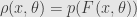
Assume we want to estimating a state $x \in R^n$ from $m \gg n$ noisy linear measurements $y \in R^m$ , $y = Ax + z$ , $z$ – noise with outliers, like in the paper by Sharon, Wright and Ma Minimum Sum of Distances Estimator: Robustness and Stability
Sharon at al show that minimum $L_1$ norm estimator, that is
$arg \min_{x} \sum_{i=1}^{m} \| a_i^T x - y_i \|_{1}$
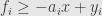
is a robust estimator with stable breakdown point, not depending on the noise level. What Sharon did was to use as cost function the sum of absolute values of all components of errors vector. However there are exists another approach.
In one-dimensional case minimum $L_1$ norm is a median.But there exist generalization of median to $R^n$ – geometric median. In our case it will be
$arg \min_{x} \sum_{i=1}^{m} \| A x - y_i \|_{2}$
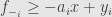
That is not a least squares – minimized the sum of $L_2$ norm, not the sum of squares of $L_2$ norm.
Now why is this a stable and robust estimator? If we look at the Jacobian
$\sum_{i=1}^{m} A^T \frac{A x - y_i}{ \| A x - y_i \|_{2}}$
we see it’s asymptotically constant, and it’s norm doesn’t depend on the norm of the outliers. While it’s not a formal proof it’s quite intuitive, and can probably be formalized along the lines of Sharon paper.
While first approach with $L_1$ norm can be solved with linear programming, for example simplex method and interior point method, the second approach with $L_2$ norm can be solved with second order cone programming and …surprise, interior point method again.
For interior point method, in both cases original cost function is replaced with
$\sum f$
And the value of $f$ is defined by constraints. For $L_1$
$f_{i} \ge a_ix-y_i$ , $f_{i} \ge -a_ix+y_i$
Sometimes it’s formulated by splitting absolute value is into the sum of positive and negative parts
$f_{+_{i}} \ge a_ix-y_i$ , $f_{-_{i}} \ge -a_ix+y_i$ , $f_{+_{i}} \ge 0$ , $f_{-_{i}} \ge 0$
And for $L_2$ it’s a simple
$f_i \ge \| A x - y_i \|_{2}$
Formulations are very similar, and stability/performance are similar too (there was a paper about it, just had to dig it out)