Some thoughts about deep learning criticism

There is some deep learning (specifically #convnet) criticism based on the artificially constructed misclassification examples.
There is a new paper
“Deep Neural Networks are Easily Fooled: High Confidence Predictions for Unrecognizable Images” by Nguen et al
http://arxiv.org/abs/1412.1897
and other direction of critics is based on the older, widely cited paper
“Intriguing properties of neural networks” by Szegedy et al
http://arxiv.org/abs/1312.6199
In the first paper authors construct examples which classified by convnet with confidence, but look nothing like label to human eye.
In the second paper authors show that correctly classified image could be converted to misclassified with small perturbation, which perturbation could be found by iterative procedure
What I think is that those phenomenons have no impact on practical performance of convolutional neural networks.

First paper is really simple to address. The real world images produced by camera are not dense in the image space(space of all pixel vectors of image size dimension).
In fact camera images belong to low-dimensional manifold in the image space, and there are some interesting works on dimensionality and property of that manifold. For example dimensionality of the space images of the fixed 3D scene it is around 7, which is not surprising, and the geodesics of that manifold could be defined through the optical flow.
Of cause if sample is outside of image manifold it will be misclassified, method of training notwithstanding. The images in the paper are clearly not real-world camera images, no wonder convnet assign nonsensical labels to them.

Second paper is more interesting. First I want to point that perturbation which cause misclassification is produced by iterative procedure. That hint that in the neighbourhood of the image perturbed misclassified images are belong to measure near-zero set.
Practically that mean that probability of this type of misclassification is near zero, and orders of magnitude less than “normal” misclassification rate of most deep networks.
But what is causing that misclassification? I’d suggest that just high dimensionality of the image and parameters spaces and try to illustrate it. In fact it’s the same reason why epsilon-sparse vector are ubiquitous in real-world application: If we take n-dimensional vector, probability that all it’s components more than is , which is near zero. This and like effects explored in depth in compressed sensing ( also very good Igor Carron’s page)
Now to convnet – convnet classify images by signs of piecewise-linear functions.
Take any effective pixel which is affecting activations. Convolutional network separate image space into piecewise-linear areas, which are not aligned with coordinate axes. That mean if we change intensity of pixel far enough we are out of correct classification area.
We don’t know how incorrect areas are distributed in the image space, but for common convolutional network dimensionality of subspace of the hyperplanes which make piecewise-linear separation boundary is several times more than dimensionality of the image vector. This suggest that correlation between incorrect areas of different pixels is quite weak.
Now assume that image is stable to perturbation, that mean that exist \epsilon such that for any effective pixel it’s epsilon-neighbourhood is in the correct area. If incorrect areas are weakly correlated that mean probability of image being stable is about , where n is number of effective pixels. That is probability of stable image is near zero. That illustrate suggestion that this “adversarial” effect is only caused by dimensionality of the problem and parameter space, not by some intrinsic deficiency of the deep network.

Geoffrey Hinton on max pooling (reddit AMA)

Geoffrey Hinton, neural networks, ML, deep learning pioneer answered “Ask Me Anything” on reddit:

AMA Geoffrey Hinton
byu/geoffhinton inMachineLearning

His answers only:
https://www.reddit.com/user/geoffhinton

His most controversial answer is:
The pooling operation used in convolutional neural networks is a big mistake and the fact that it works so well is a disaster.
If the pools do not overlap, pooling loses valuable information about where things are. We need this information to detect precise relationships between the parts of an object. Its true that if the pools overlap enough, the positions of features will be accurately preserved by “coarse coding” (see my paper on “distributed representations” in 1986 for an explanation of this effect). But I no longer believe that coarse coding is the best way to represent the poses of objects relative to the viewer (by pose I mean position, orientation, and scale).
I think it makes much more sense to represent a pose as a small matrix that converts a vector of positional coordinates relative to the viewer into positional coordinates relative to the shape itself. This is what they do in computer graphics and it makes it easy to capture the effect of a change in viewpoint. It also explains why you cannot see a shape without imposing a rectangular coordinate frame on it, and if you impose a different frame, you cannot even recognize it as the same shape. Convolutional neural nets have no explanation for that, or at least none that I can think of.

It’s interesting though controversial opinion, and here is my take on it:
It looks like Convolutional networks discriminate input by switching between activation subnetworks (http://arxiv.org/abs/1410.1165, Understanding Locally Competitive Networks)
From that point of view max pooling operation is pretty natural – it provide both robustness to small deviations and switching between activation subsets. Aslo max pooling has a nice property to be semilinear to multiplication f(ax)=af(x) , which make all the layers stack but last cost layer semilinear, and if one use SVM/L2SVM as cost whole stack semilinear. Not sure if it help in discrimination, but it surely help in debugging.
As alternative to pooling pyramid Geoffrey Hinton suggest to get somehow global rotation(or other transformation) matrix from the image.
Getting it from image or from image patch is actually possible with low-rank matrix factorization from single image(Transform Invariant Low-rank Textures by Zhang et al) and by optical flow (or direct matching) from set of images, but it’s quite expensive in performance term. It’s definitely possible to combine those method with deep network, (ironically they are benefit using pooling pyramid)
but:
1. They will be kind of image augmentation
2. Those are problem-specific methods, they may not help in other domains like NLP, speech etc.

There are some work on using low-rank matrix factorization in deep networks, but they are mostly about fully connected, not convolutional layers. But IMHO if to try do factorization in conv layers, the pooling wouldn’t go away.

PS (edit): Here is a video with Hinton alternative to pooling – “capsules”
http://techtv.mit.edu/collections/bcs/videos/30698-what-s-wrong-with-convolutional-nets

November finds in #arxiv and NIPS 2013

This is “find in arxiv” reposts form my G+ stream for November.

NIPS 2013

Accelerating Stochastic Gradient Descent using Predictive Variance Reduction

Stochastic gradient (SGD) is the major tool for Deep Learning. However if you look at the plot of cost function over iteration for   SGD you will see that after quite fast descent it becoming extremely slow, and error decrease could even become non-monotonous.  Author explain by necessity of trade of between the step size and variance of random factor – more precision require smaller variance but that mean smaller descent step and slower convergence. “Predictive variance” author suggest to mitigate problem is the same old “adding back the noise” trick, used for example in Split Bregman. Worth reading IMHO.

http://papers.nips.cc/paper/4937-accelerating-stochastic-gradient-descent-using-predictive-variance-reduction

Predicting Parameters in Deep Learning
Output of the first layer of ConvNet is quite smooth, and that could be used for dimensionality reduction, using some dictionary, learned or fixed(just some simple kernel). For ConvNet predicting 75% of parameters with fixed dictionary have negligible effect on accuracy.
http://papers.nips.cc/paper/5025-predicting-parameters-in-deep-learning

Learning a Deep Compact Image Representation for Visual Tracking
Application of ADMM (Alternating Direction Method of Multipliers, of which Split Bregman again one of the prominent examples) to denoising autoencoder with sparsity.
http://papers.nips.cc/paper/5192-learning-a-deep-compact-image-representation-for-visual-tracking

Deep Neural Networks for Object Detection
People from Google are playing with Alex Krizhevsky’s ConvNet
http://papers.nips.cc/paper/5207-deep-neural-networks-for-object-detection

–arxiv (last)–

Are all training examples equally valuable?
It’s intuitively obvious that some training sample are making training process worse. The question is – how to find wich sample should be removed from training? Kind of removing outliers. Authors define “training value” for each sample of binary classifier.
http://arxiv.org/pdf/1311.7080

Finding sparse solutions of systems of polynomial equations via group-sparsity optimization
Finding sparse solution of polynomial system with lifting method.
I still not completely understand why quite weak structure constraint is enough for found approximation to be solution with high probability. It would be obviously precise  for binary 0-1 solution, but why for general sparse?
http://arxiv.org/abs/1311.5871

Semi-Supervised Sparse Coding
Big dataset with small amount of labeled samples – what to do? Use unlabeled samples for sparse representation. And train labeled samples in sparse representation.
http://arxiv.org/abs/1311.6834
From the same author, similar theme – Cross-Domain Sparse Coding
Two domain training – use cross domain data representation to map all the samples from both source and target domains to a data representation space with a common distribution across domains.
http://arxiv.org/abs/1311.7080

Robust Low-rank Tensor Recovery: Models and Algorithms
More of tensor decomposition with trace norm
http://arxiv.org/abs/1311.6182

Complexity of Inexact Proximal Newton methods
Application of Proximal Newton (BFGS) to subset of coordinates each step – active set coordinate descent.
http://arxiv.org/pdf/1311.6547

Computational Complexity of Smooth Differential Equations
Polynomial-memory complexity of ordinary differential equations.
http://arxiv.org/abs/1311.5414

–arxiv (2)–

Deep Learning

Visualizing and Understanding Convolutional Neural Networks
This is exploration of Alex Krizhevsky’s  ConvNet
( https://code.google.com/p/cuda-convnet/ )
using “deconvnet” approach – using deconvolution on output of each layer and visualizing it. Results looks interesting – strting from level 3 it’s something like thersholded edge enchantment, or sketch. Also there are evidences supporting “learn once use everywhere” approach – convnet trained on ImageNet is also effective on other datasets
http://arxiv.org/abs/1311.2901

Unsupervised Learning of Invariant Representations in Hierarchical Architectures
Another paper on why and how deep learning works.
Attempt to build theoretical framework for invariant features in deep learning. Interesting result – Gabor wavelets are optimal filters for simultaneous scale and translation invariance. Relations to sparsity and scattering transform
http://arxiv.org/abs/1311.4158

Computer Vision
An Experimental Comparison of Trust Region and Level Sets
Trust regions method for energy-based segmentation.
Trust region is one of the most important tools in optimization, especially non-convex.
http://en.wikipedia.org/wiki/Trust_region
http://arxiv.org/abs/1311.2102

Blind Deconvolution with Re-weighted Sparsity Promotion
Using reweighted L2 norm for sparsity in blind deconvolution
http://arxiv.org/abs/1311.4029

Optimization

Online universal gradient methods
about  Nesterov’s universal gradient method (
http://www.optimization-online.org/DB_FILE/2013/04/3833.pdf )
It use Bregman distance and related to ADMM.
The paper is application of universal gradient method  to online learning and give bound on regret function.
http://arxiv.org/abs/1311.3832

CS
A Component Lasso
Approximate covariance matrix with block-diagonal matrix and apply Lasso to each block separately
http://arxiv.org/abs/1311.4472

_FuSSO: Functional Shrinkage and Selection Operator
Lasso in functional space with some orthogonal basis_
http://arxiv.org/abs/1311.2234

Non-Convex Compressed Sensing Using Partial Support Information
More of Lp norm for sparse recovery. Reweighted this time.
http://arxiv.org/abs/1311.3773

–arxiv  (1)–

Optimization, CS
Scalable Frames and Convex Geometry
Frame theory is a basis(pun intended) of wavelets theory, compressed sening and overcomplete dictionaries in ML
http://en.wikipedia.org/wiki/Frame_of_a_vector_space
Here is a discussion how to make “tight frame”
http://en.wikipedia.org/wiki/Frame_of_a_vector_space#Tight_frames
from an ordinary frame by scaling m of its components
Interesting geometric insight provided – to do it mcomponents of frame should make “blunt cone”
http://en.wikipedia.org/wiki/Convex_cone#Blunt_and_pointed_cones
http://arxiv.org/abs/1310.8107

Learning Sparsely Used Overcomplete Dictionaries via Alternating Minimization
Some bounds for convergence of dictionary learning. Converge id initial error is O(1/s^2), s- sparcity level
http://arxiv.org/abs/1310.7991

Robust estimators
Robustness of ℓ1 minimization against sparse outliers and its implications in Statistics and Signal Recovery
This is another exploration of L1 estimator. It happens (contrary to common sense) that L1 is not especially robust from “breakdown point” point of view if there is no constraint of noise. However it practical usefulness can be explained that it’s very robust to sparse noise
http://arxiv.org/abs/1310.7637

Numerical
Local Fourier Analysis of Multigrid Methods with Polynomial Smoothers and Aggressive coarsening
Overrelaxaction with Chebyshev weights on the fine grid, with convergence analysis.
http://arxiv.org/abs/1310.8385

Meaning of conditional probability

Conditional probability was always baffling me. Empirical, frequentists meaning is clear, but the abstract definition, originating from Kolmogorov – what was its mathematical meaning? How it can be derived? It’s a nontrivial definition and is appearing in the textbooks out the air, without measure theory intuition behind it.

Here I mostly follow Chang&Pollard  paper  Conditioning as disintegartion. Beware that the paper use non-standard notation, but this post follow more common notation, same as in wikipedia.

Here is example form Chang&Pollard paper:

Suppose we have distribution on   concentrated in two straight lines  and  with respective density  and angles with X axis . Observation (X,Y) taken, giving , what is probability that point lies on the line  ?

Standard approach would be approximate  with  and take limit with  

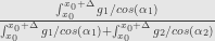
Not only taking this limit is kind of cumbersome, it’s also not totally obvious that it’s the same conditional probability that defined in the abstract definition – we are replacing ratio with limit here.

Now what is “correct way” to define conditional probabilities, especially for distributions?

Disintegration!

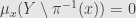
For simplicity we will first talk about single scalar random variable, defined on probability space. We will think of random variable X as function on the sample space. Now condition define fiber – inverse image of .

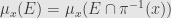
Disintegration theorem say that probability measure on the sample space can be decomposed into two measures – parametric family of measures induced by original probability on each fiber and “orthogonal” measure on  – on the parameter space of the first measure. Here is the space of values of X  and serve as parameter space for measures on fibers. Second measure induced by the inverse image of  the function (random variable) for each measurable set on . This second measure is called Pushforward measure. Pushforward measure is just for measurable set on (in our case) taking its X  inverse image on sample space and measuring it with μ.

Fiber is in fact sample space for conditional event, and measure on fiber is our conditional distribution.

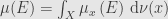
Full statement of the theorem require some term form measure theory. Following wikipedia

Let P(X) is collection of Borel probability measures on X,  P(Y) is collection of  Borel probability measures on Y

Let Y and X be two Radon spaces. Let μ ∈ P(Y), let : Y → X be a Borel- measurable function, and let ν ∈ P(X) be the pushforward measure  .

* Then there exists a ν-almost everywhere uniquely determined family of probability measures  ⊆  P(Y) such that
* the function is Borel measurable, in the sense that is a Borel-measurable function for each Borel-measurable set B ⊆ Y;
*    “lives on” the  fiber  : for ν-almost all x  ∈ X,

and so

* for every Borel-measurable function : Y → [0, ∞],

From here for any event E form Y

This was complete statement of the disintegration theorem.

Now returning to Chang&Pollard example. For formal derivation I refer you to the original paper, here we will just “guess” , and by uniqueness it give us disintegration. Our conditional distribution for  will be just point masses on the intersections of lines and  with axis  
Here is delta function – point mass.

and for

Our conditional probability that event lies on with condition , form conditional density thus

Another example from Chen&Pollard. It relate to sufficient statistics. Term sufficient statistic used if we have probability distribution depending on some parameter, like in maximum likelihood estimation. Sufficient statistic is some function of sample, if it’s possible to estimate parameter of distribution from only values of that function in the best possible way – adding more data form the sample will not give more information about parameter of distribution.
Let be uniform distribution on the square . In that case M = max(x, y) is sufficient statistics for . How to show it?
Let take our function , and make disintegration.
is a uniform distribution on edges where x and y equal m and
is density of conditional probability and it doesn’t depend on
For any – means that M is  sufficient.

It seems that in most cases disintegration is not a tool for finding conditional distribution. Instead it can help to guess it and form uniqueness prove that the guess is correct. That correctness could be nontrivial – there are some paradoxes similar to Borel Paradox in Chang&Pollard paper.