2013 January « Mirror Image

Split-Bregman for total variation: parameter choice

Split Bregamn method is one of the most used method for solving convex optimization problem with non-smooth regularization. Mostly it used for $L_1$ regularization, and here I want to talk about TV-L1 and similar regularizers ( like $\|\Psi u\|_1$ )
For simplest possible one-dimentional denoising case
$min_{u} \quad (u-f)^2 - \mu\|\frac{\partial u}{\partial x}\|_1$ (1)
Split Bregman iteration looks like
$min_{\substack u} \quad (u-f)^2 + \mu\lambda(\frac{\partial u}{\partial x}+b-d)^2$ (2)
$d = Shrink(\frac{\partial u}{\partial x} + b, \frac{1}{\lambda})$ (3)
$b = b + \frac{\partial u}{\partial x} - d$ (4)
There is a lot of literature about choosing $\mu$ parameter from (1) for denosing. Methods include Morozov discrepancy principle, L-curve and more – that’s just parameter of Tikhonov regularization.
There is a lot less metods for choosing $\lambda$ for Split Bregman.
Theoretically $\lambda$ shouldn’t be very important – if Split Bregman converge solution is not depending on $\lambda$ . In practice of cause convergence speed and stability depend on $\lambda$ a lot. Here I’ll point out some simple consideration which may help to choose $\lambda$
Assume for simplicity that u is twice differentiable almoste everythere, the (1) become
$Lu = u-f - \mu\lambda*(\frac{\partial^2 u}{\partial x^2} + \frac{\partial b}{\partial x} - \frac{\partial d}{\partial x}) = 0$ (5)
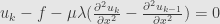
We know if Split Bbregman converge $d \to \frac {\partial u}{\partial x}$
that mean $\frac {\partial b} {\partial x} \to \frac {\partial} {\partial x} sign(\frac {\partial u}{\partial x})$ , here exteranl derivative is a weak derivative.
For the solution b is therefore locally constant, and we even know what constant it is.
Recalling
$Shrink(x, \frac{1}{\lambda}) = \left\{\begin{array} {l l} |x| \leq \frac{1}{\lambda} : 0\\ |x| > \frac{1}{\lambda} : x - sign(x)\frac{1}{\lambda} \end{array} \right.$
For $|x| > \frac{1}{\lambda}$ we have
$d = \frac{\partial u}{\partial x} + b \pm \frac{1}{\lambda}$
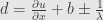
and accordingly
$b = \mp \frac{1}{\lambda}$
For converged solution
$b(x) = \frac{1}{\lambda}sign(\frac{\partial u}{\partial x})$
everythere where $\frac {\partial u}{\partial x}$ is not zero, with possible exeption of measure zero set.
Now returning to choice of $\lambda$ for Split Bregman iterations.
From (4) we see that for small values b , b grow with step $\frac {\partial u}{\partial x}$ until it reach it’s maximum absolute value $\pm \frac{1}{\lambda}$
Also if the b is “wrong”, if we want for it to switch value in one iteration $| \frac {\partial u}{\partial x}|$ should be more than $\frac{2}{\lambda}$
That give us lower boundary for $\lambda$ :
For most of x $| \frac {\partial u}{\partial x}| \geq \frac{2}{\lambda}$
What happens if on some interval b reach $\mp \frac{1}{\lambda}$ for two consequtive iterations?
Then on the next iteration form (5) and (3) on that interval
$u_k-f - \mu\lambda(\frac{\partial^2 u_k}{\partial x^2}-\frac{\partial^2 u_{k-1}}{\partial x^2} ) = 0$
or
$u_k = min_{u} (u-f)^2 + \mu\lambda(\frac {\partial u}{\partial x} - \frac {\partial u_{k-1}}{\partial x})^2$
See taht with $\mu\lambda$ big enuogh sign of $\frac {\partial u_k}{\partial x}$ stabilizing with high probaility and we could be close to true solution. The “could” in the last sentence is there because we are inside the interval, and if the values of u on the ends of interval are wrong b “flipping” can propagate inside our interval.
It’s more difficult to estimate upper boundary for $\lambda$ .
Obviously for more easy solution of (2) or (5) $\lambda$ shouldn’t be too big, so that eigenvalues of operator $L$ woudn’t be too close to 1. Because solutions of (2) are inexact in Split Breagman we obviously want $L$ having bigger eigenvalues, so that single (or small number of) iteration could suppress error good enough for (2) subproblem.
So in conclusion (and my limited experience) if you can estimate $avg |\frac {\partial u}{\partial x}|$ for solution $\lambda = \frac{2}{avg |\frac {\partial u}{\partial x}|}$ could be a good value to start testing.