Deriving Gibbs distribution from stochastic gradients
Stochastic gradients is one of the most important tools in optimization and machine learning (especially for Deep Learning – see for example ConvNet). One of it’s advantage is that it behavior is well understood in general case, by application of methods of statistical mechanics.
In general form stochastic gradient descent could be written as
where 
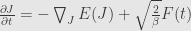
To apply methods of statistical mechanics we can rewrite it in continuous form, as stochastic gradient flow
and random variable F(t) we assume to be white noise for simplicity.
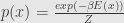
In that moment most of textbooks and papers refer to “methods of statistical mechanics” to show that
stochastic gradient flow has invariant probability distribution, which is called Gibbs distribution
and from here derive some interesting things like temperature and free energy.
The question is – how Gibbs distribution derived from stochastic gradient flow?


First we have to understand what stochastic gradient flow really means.
It’s not a partial differential equation (PDE), because it include random variable, which is not a function 
SDE in question is called Ito diffusion. Solution of that equation is a stochastic process – collection of random variables parametrized by time. Sample path of stochastic process in question as a function of time is nowhere differentiable – it’s difficult to talk about it in term of derivatives, so it is defined through it’s integral form.
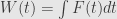
First I’ll notice that integral of white noise is actually Brownian motion, or Wiener process.
Assume that we have stochastic differential equation written in informal manner

It’s integral form is
where W(t) is a Wiener process
This equation is usually written in the form
This is only a notation for integral equation, d here is not a differential.
Returning to (1)


The most notable thing here is

It’s a stochastic integral, and it’s defined in the courses of stochastic differential equation as the limit of Riemann sums of random variables, in the manner similar to definition of ordinary integral.
Curiously, stochastic integral is not quite well defined. Depending on the form of the sum it produce different results, like Ito integral:
Different Riemann sums produce different integral – Stratonovich integral:
![\int_0^t g \,d W =\lim_{n\rightarrow\infty} \sum_{[t_{i-1},t_i]\in\pi_n}g_{t_{i-1}}(W_{t_i}-W_{t_{i-1}})](https://s0.wp.com/latex.php?latex=%5Cint_0%5Et+g+%5C%2Cd+W+%3D%5Clim_%7Bn%5Crightarrow%5Cinfty%7D+%5Csum_%7B%5Bt_%7Bi-1%7D%2Ct_i%5D%5Cin%5Cpi_n%7Dg_%7Bt_%7Bi-1%7D%7D%28W_%7Bt_i%7D-W_%7Bt_%7Bi-1%7D%7D%29&bg=e6e6e6&fg=333333&s=0&c=20201002)
![\int_0^t g \,d W =\lim_{n\rightarrow\infty} \sum_{[t_{i-1},t_i]\in\pi_n}(g_{t_i} + g_{t_{i-1}})/2(W_{t_i}-W_{t_{i-1}})](https://s0.wp.com/latex.php?latex=%5Cint_0%5Et+g+%5C%2Cd+W+%3D%5Clim_%7Bn%5Crightarrow%5Cinfty%7D+%5Csum_%7B%5Bt_%7Bi-1%7D%2Ct_i%5D%5Cin%5Cpi_n%7D%28g_%7Bt_i%7D+%2B+g_%7Bt_%7Bi-1%7D%7D%29%2F2%28W_%7Bt_i%7D-W_%7Bt_%7Bi-1%7D%7D%29&bg=e6e6e6&fg=333333&s=0&c=20201002)
Ito integral used more often in statistics because it use 
Returning to Ito integral – Ito integral is stochastic process itself, and it has expectation zero for each t.
From definition of Ito integral follow one of the most important tools of stochastic calculus – Ito Lemma (or Ito formula)
Ito lemma states that for solution of SDE (2)

were W is Wiener process (actually some more general process) and b and g are good enough

where 
From Ito lemma follow Ito product rule for scalar processes: applying Ito formula to process 
Using Ito formula and Ito product rule it is possible to get Feynman–Kac formula (derivation could be found in the wikipedia, it use only Ito formula, Ito product rule and the fact that expectation of Ito integral (3) is zero):
for partial differential equation (PDE)
with terminal condition
solution can be written as conditional expectation:
Feynman–Kac formula establish connection between PDE and stochastic process.
From Feynman–Kac formula taking 

for
equation
with terminal condition (4) have solution as conditional expectation
From Kolmogorov backward equation we can obtain Kolmogorov forward equation, which describe evolution of probability density for random process X (2)
In SDE courses it’s established that (2) is a Markov process and has transitional probability P and transitional density p:
p(x, s, y, t) = probability density at being at y in time t, on condition that it started at x in time s
taking u – solution of (5) with terminal condition (6)
From Markov property
from here
form here
from (5)
Now we introduce dual operator
By integration by part we can get
and from (7)
for t=T
This is true for any 
And we get Kolmogorov forward equation for p. Integrating by x we get the same equation for probability density at any moment T
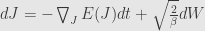
Now we return to Gibbs invariant distribution for gradient flow
Stochastic gradient flow in SDE notation
We want to find invariant probability density 
so from Kolmogorov forward equation
or
removing gradient
C = 0 because we want
and at last we get Gibbs distribution
Recalling again the chain of reasoning:
Wiener process →


![u(x,t) = E\left[ \int_t^T e^{- \int_t^r v(X_\tau,\tau)\, d\tau}f(X_r,r)dr + e^{-\int_t^T v(X_\tau,\tau)\, d\tau}\psi(X_T) \Bigg| X_t=x \right]](https://s0.wp.com/latex.php?latex=u%28x%2Ct%29+%3D+E%5Cleft%5B+%5Cint_t%5ET+e%5E%7B-+%5Cint_t%5Er+v%28X_%5Ctau%2C%5Ctau%29%5C%2C+d%5Ctau%7Df%28X_r%2Cr%29dr+%2B+e%5E%7B-%5Cint_t%5ET+v%28X_%5Ctau%2C%5Ctau%29%5C%2C+d%5Ctau%7D%5Cpsi%28X_T%29+%5CBigg%7C+X_t%3Dx+%5Cright%5D+&bg=e6e6e6&fg=333333&s=0&c=20201002)


SDE + Ito Lemma + Ito product rule + zero expecation of Ito integral →
Kolmogorov backward equation + Markov property of SDE →
Kolmogorov forward equation for probability density →
ConvNet for windows
I have seen an excellent wlakthrough on building Alex Krizhevsky’s cuda-convnet for windows, but difference in configuration and installed packages could be tiresome. So here is complete build of convnet for windows 64:
https://github.com/s271/win_convnet
It require having CUDA compute capability 2.0 or better GPU of cause, Windows 64bit, Visual Studio 64bits and Python 64bit with NumPy installed. The rest of libs and dlls are precomplied. In building it I’ve followed instructions by Yalong Bai (Wyvernbai) from http://www.asiteof.me/archives/50.
Read Readme.md before installation – you may (or may not) require PYTHONPATH environmental variable set.
On side note I’ve used WinPython for both libraries and running the package. WinPython seems a very nice package, which include Spyder IDE. I have some problems with Spyder though – sometimes it behave erratically during debugging/running the code. Could be my inexperience with Spyder though. Another nice package – PythonXY – regretfully can not be used – it has only 32 bit version and will not compile with/run 64 bit modules.
__volatile__ in #cuda reduce sample
“Reduce” is one of the most useful samples in NVIDIA CUDA SDK. It’s implementation of highly optimized cuda algorithm for some of the elements of the array of the arbitrary length. It’s hardly possible to make anything better and generic enough with existing GPGPU architecture (if anyone know something as generic but considerably more efficient I’d like to know too). One of the big plus of the reduce algorithm is that it can work for any binary commutative associative operation – like min, max, multiply etc. And NVIDIA sample provide this ability – it’s implemented as reduce on template class, so all one have to do is implement class with overload of addition and assignment operations.
However there is one obstacle – it’s a __volatile__ qualifier in the code. Simple overload of “=” “+=” and “+” operations in class LSum cause compiler error like
error: no operator “+” matches these operands
1> operand types are: LSum + volatile LSum
The answer is add __volatile__ to all class operation, but there is the trick here:
for “=” just
volatile LSum& operator =(volatile LSum &rhs)
is not enough. You should add volatile to the end too, to specify not only input and output, but function itself as volatile.
At the end class looks like:
class LSum
{
public:
…
__device__ LSum& operator+=(volatile LSum &rhs)
{
…
return *this;
};
__device__ LSum operator+(volatile LSum &rhs)
{
LSum res = *this;
res += rhs;
return res;
};
__device__ LSum& operator =(const float &LSum)
{
…
return *this;
};
__device__ volatile LSum& operator =(volatile LSum &rhs) volatile
{
…
return *this;
};
};
Algebraic topology – now in compressed sensing
Thanks to Igor Carron for pointing me to this workshop – Algebraic Topology and Machine Learning . There is very interesting paper there Persistent Homological Structures in Compressed Sensing and Sparse Likelihood by Moo K. Chung, Hyekyung Lee and Matthew Arnold. The paper is very comprehensive and require only minimal understanding of some algebraic topology concepts (which is exactly where I’m in realation to algebraic topology). Basically it’s application of topological data analysis to compressive sensing. They use such thing as persistent homology and “barcodes”. Before, persistent homology and barcodes were used for such things as extracting solid structure from noisiy point cloud. Barcode is stable to noise dependence of some topological invariants on some parameter. In case of point cloud parameter is the radius of the ball around each point. As radius go from very big to zero topology of union of balls change, and those changes of topology make barcode. Because barcode is stable topological invariant learning barcode is the same as learning topology of solid structure underlying point cloud.
In the paper authors using graphical lasso (glasso) with 

PS Using this approach for total variation denoising barcode would include dependance of size function from smoothing parameter.
Total Variation in Image Processing and classical Action
This post is inspired by Extremal Principles in Classical, Statistical and Quantum Mechanics in Azimuth blog.
Total Variation used a lot in image processing. Image denoising, optical flow, depth maps processing. The standard form of Total Variation f or 
(I’m talking about Total Variaton-
In case of image denoising it would be
where 

Part 

Regularizer part is to provide smoothness of solution and fidelity term is to force smooth solution to resemble original image (that is in case of image denoising)
Now if we return to classical Action, movement of the point is defined by the minimum of functional


One-dimensional
Of cause the strict equality hold only for one-dimentional image and
While it hold some practical meaning, most of practical task have two or more dimensional image and 
which has uncanny resemblance to Lagrangian of relativistic particle
So total variation in image processing is equivalent to physics of non-classical movement with multidimensional time, in the field with potential energy defined by image. I have no idea what does it signify, but it sounds cool :) . Holographic principle? May be crowd from Azimuth or n-category cafe will give some explanation eventually…
And another, related question: regularizer in Total Variation. There is inherent connection between regularizers and Bayesian priors. What TV-L1 regularizer mean from Bayesian statistics point of view?


PS I’m posting mostly on my google plus now, so this blog is a small part of my posts.
Stuff and AR
I once asked, what’s 3d registration/reconstruction/pose estimation is about – optimization or statistics? The more I think about it, the more I convinced it’s at least 80% statistics. Often specifically optimization tricks like Tikhonov regularization have statistical underpinning. Stability of optimization is robust statistics(Yes I know, I repeat it way too often). Cost function formulation is a formulation for error distribution and define convergence speed.
Now unrelated(almost) AR stuff:
I already mentioned on Twitter that version of markerless tracker for which I did a lot of work is part of Samsung AR SDK (SARI) for Android and Bada. It was was shown at AP2011(Presentaion and also include nice Bada code). AR SDK presentation is here.
Some videos form presentation – Edi Bear game demo with non-reference tracking at the end of the video and less trivial elements of SLAM tracking. Other application of SARI SDK – PBI (This one seems use earlier version).
How Kinect depth sensor works – stereo triangulation?
Kinect use depth sensor produced by PrimeSense, but how exactly it works is not obvious from the first glance. Some person here, claimed to be specialist, assured me that PrimeSense sensor is using time-of-flight depth camera. Well, he was wrong. In fact PrimeSense explicitly saying they are not using time-of-flight, but something they call “light coding” and use standard off-the shelf CMOS sensor which is not capable extract time of return from modulated light.
Daniel Reetz made excellent works of making IR photos of Kinect laser emitter and analyzing it’s characteristics. He confirm PrimeSense statement – IR laser is not modulated. All that laser do is project static pseudorandom pattern of specs on the environment. PrimeSense use only one IR sensor. How it possible to extract depth information from the single IR image of the spec pattern? Stereo triangulation require two images to get depth of each point(spec). Here is the trick: actually there not one, but two images. One image is what we see on the photo – image of the specs captured by IR sensor. The second image is invisible – it’s a hardwired pattern of specs which laser project. That second image should be hardcoded into chip logic. Those images are not equivalent – there is some distance between laser and sensor, so images correspond to different camera positions, and that allow to use stereo triangulation to calculate each spec depth.

The difference here is that the second image is “virtual” – position of the second point y_2 is already hardcoded into memory. Because laser and sensor are aligned that make task even more easy: all one have to do is to measure horizontal offset of the spec on the first image relative to hardcoded position(after correcting lens distortion of cause).
That also explain pseudorandom pattern of the specs. Pseudorandom patten make matching of specs in two images more easy, as each spec have locally different neighborhood. Can it be called “structured light” sensor? With some stretch of definition. Structured light usually project grid of regular lines instead of pseudorandom points. At least PrimeSense object to calling their method “structured light”.
New laptop, new Ubuntu
Got myself new and shiny Asus u35jc-a1 and started dual boot Ubuntu on it. I have ubuntu as wubi(ubuntu in windows file) on my old desktop replacement Dell XPS, so I started with wubi for u35jc too. Wubi worked from the start, wifi card works without problem. However NVIDIA completely screwed up hybrid driver for Linux(there are 2 vidoecards on u35jc, one integrated and other NVIDIA), it’s completely unusable, so NVIDIA driver should be disabled. Happily there are detailed instructions on ubuntuforums. They are for 10.4, but work for 10.10 too. Suspend was not working quite stable though, even after fix from ubuntuforums. It’s tricky – suspension require turing NVIDIA driver on and off.. Suspend was working for AC power, but suspend on battery power caused system hang someteimes. I proceed to multituch fix from the list. Multituch fix require creation or modification of xorg.conf, wich require stopping X. Stopping X caused crush which permanently killed Ubuntu wubi install. That was quite scary, so I decided to forgo wubi and make complete ubuntu intallation into partition.
Installation was not completely smooth. Probably because of some quirks of initial Asus partition, ubuntu installer refused to create any partition but first in the free space. After creation of the first boot partition remaining free disk space become unusable. So I forgo swap partition and installed ubuntu into single / partition. After that I implemented only acpi_call and suspend fixes. Suspend now works like charm, both for AC and battery. Multitach fix I put aside for now – it’s not critical. It seems all the problem, necessity of separate suspend fix, problems with wubi and stopping X were caused by NVIDA driver. Hope NVIDIA will fix it eventually – I want to play with GPGPU without going into Windows boot.
Is Ouidoo a rebranded Zii Egg?
There ii some buzz on the net about a new smartphone specifically designed for augmented reality – Ouidoo. Some of the specs of the device sound outlandish – 26 CPUs, 8 GFLOPS and a new OS.
However one commenter on the cn.engadged.com pointed out that this device could actually be real – it specs resemble that of the new Creative Zii Egg OEM platform, which seems available for developers now. Zii Egg feature a new OS -“Plasma OS”, but also support Android. So what’s the deal with 26 CPUs?
Those are not general-propose CPUs of cause, but Zii Egg have some kind of vector processor (like in Cell processor or modern GPUs, some high-end smartphones also have it) with 24 floating point units. Add to this CPU itself – ARM Coretx8 and possibly dedicated GPU and you have 24+1+1 = 26. Also specs claimed by Creative for Zii Egg floating point vector processor – 8 GFLOPS are exactly those clamied by QderoPateo for Ouidoo.
